Soft Actor Critic (SAC) is a model-free Reinforcement Learning (RL) method developed by Tuomas Haarnoja in a series of papers culminating in Soft Actor-Critic Algorithms and Applications. It is one of the seminal RL papers for continuous control and has inspired much of my work. In this blog post, I’ll review the theory and derivation behind SAC from zero to a fully-derived algorithm without skipping (almost) any of the mathematical details. This time I haven’t included an implementation of my own, but a good one to go along with this blog post is denisyarats/pytorch_sac.
Note: If you are familiar with RL basics, feel free to skip ahead
Table of contents
- Problem
- Bellman Equations
- TD Learning
- Q-Learning
- Policy Gradients
- Actor critic methods
- Soft Actor Critic
- Soft Actor Critic with automatic temperature
- Refernces
- Further resources
- Acknowledgements
Problem
We want a robot with limited perceptive abilities to learn to achieve a given task. Let’s formulate this mathematically and ground it in the real world via a beer-opening robot:
- The world has a state at a given time $s_t \in S$. This state space can consist of anything meaningful to the robot: the position of the beer bottle? how full is it? how thirsty is the human we need to serve?
- Unfortunately, robots can’t open beer bottles by just thinking about it really hard; instead, they have to act in the world via actions $a_t \in A$. For our robot, actions could be a 4-dimensional torque vector to control all robot arm joints.
- To incentivise the robot to achieve its goal, we give it a reward for each timestep $r_t \in \mathbb{R}$. This could be a function of the state and action $r_t := r(s_t, a_t)$ or something more abstract like our human telling us how happy they are. The critical assumption is that the robot only gets a scalar reward $r_t$ at each timestep without knowing how it is calculated.

The goal of our agent now is to maximize the cumulative reward by choosing the optimal sequence of actions:
\[\max_{a_0, a_1, ..., a_T} \sum_{t=0}^T r_t\]
Note on horizons
To be precise, this is called a finite-horizon problem as we are only considering rewards up to a fixed timestep $T$. Naturally, this has its limitations, and often we want to consider infinite-horizon problems. Although most of the content of this blog applies to such problems, the theory is more difficult to develop.
Technically our reward can depend on several factors from previous timesteps (e.g. did the human think I look cool while opening their beer). However, that quickly becomes an exponentially more complex problem, especially theoretically. To make the problem more tractable and our lives easier, we will make an assumption:
Assumption 1: Given a sequence of state-action pairs $(s_t, a_t) \ \ \ \forall t \in [0, T]$, the transition distribution is fully defined by $p(s_{t+1} | s_t, a_t)$. This is known as the Markov Assumption.
In English: the last state $s_t$ contains all the useful information for our problem. From this we automatically get:
Corollary 1: The reward is defined as a function of our state and action $r: S \times A \rightarrow \mathbb{R}$
Visually this can be look as the following Markov Chain:
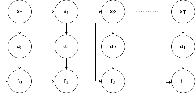
With this assumption we can now redefine our objective function as
\[\max_{a_0, a_1, ..., a_T} \sum_{t=0}^T r(s_t, a_t)\]Still, this is incorrectly defined. Why? Because we defined our transition dynamics as a probabilistic distribution in Assumption 1. To tackle that, we have to define our objective above as an expectation over the rewards:
\[\max_{a_0, a_1, ..., a_T} \sum_{t=0}^T \mathbb{E}_{s_{t+1} \sim p(s_{t} | s_{t-1}, a_{t-1})} \big[ r(s_t, a_t) \big]\]Since we’re already dealing with probabilistic distributions and ultimately want our results to fit in modern machine learning, we can constrain our actions to be coming from a set of possible policies:
Assumption 2: Actions are sampled from a probabilistic feedback policy $\pi$ parametarised by $\theta \in \mathbb{R}^d$ and conditioned only on the current state $s_t$:
\[a_t \sim \pi(a_t | s_t; \theta)\]Thus our final (and I mean it this time) objective becomes
\[\begin{equation} \max_{\theta} \sum_{t=0}^T \mathbb{E}_{s_{t+1} \sim p(s_{t} | s_{t-1}, a_{t-1}) \atop a_t \sim \pi(a_t | s_t; \theta)} \big[ r(s_t, a_t) \big] \end{equation}\]Bellman Equations
These problems get really messy really fast. Luckily we have a simple unified way to think about these problems - via the lens of value functions:
Definition 1: The value of a state $s_t$ following policy $\pi$ is given by
\[\begin{equation} V^\pi(s_t) = \sum_{n=t}^T \mathbb{E}_{s_{n+1} \sim p(s_{n} | s_{n-1}, a_{n-1}) \atop a_n \sim \pi(a_n | s_n; \theta)} \big[ r(s_n, a_n) \big] \end{equation}\]English: This is the reward we expect to receive continuing from our current state $s_t$. We will refer to this as the value function.
Let’s expand this and see where we end up
\[\begin{align} V^\pi(s_t) & = \notag \sum_{n=t}^T \mathbb{E}_{s_{n+1} \sim p(s_{n} | s_{n-1}, a_{n-1}) \atop a_n \sim \pi(a_n | s_n; \theta)} \big[ r(s_n, a_n) \big] \\ &= \notag \mathbb{E}_{a_t \sim \pi(a_t | s_t; \theta)} \bigg[ r(s_t, a_t) + \sum_{n=t+1}^T \mathbb{E}_{s_{n+1} \sim p(s_{n} | s_{n-1}, a_{n-1}) \atop a_n \sim \pi(a_n | s_n; \theta)} \big[ r(s_n, a_n) \big] \bigg] \\ &= \mathbb{E}_{a_t \sim \pi(a_t | s_t; \theta)} \bigg[ r(s_t, a_t) + \mathbb{E}_{s_{t+1} \sim p(s_{t+1} | s_{t}, a_{t})} \big[ V^\pi (s_{t+1}) \big] \bigg] \end{align}\]This recursive relationship is known as the Bellman Equation and will be key to our future derivations.
There is also another way to look at our value function from Definition 1 through the lens of an already taken action:
Definition 2: The value of a state-action pair $(s_t, a_t)$ following policy $\pi$ is given by:
\[\begin{equation} Q^\pi(s_t, a_t) = r(s_t, a_t) + \sum_{n=t+1}^T \mathbb{E}_{s_n \sim p(s_{n} | s_{n-1}, a_{n-1}) \atop a_n \sim \pi(a_n | s_n; \theta)} \big[ r(s_n, a_n) \big] \end{equation}\]We will refer to this as the state-action value function or Q function.
Similarly to value function, here we also have a recursive relationship:
\[\begin{aligned} Q^\pi(s_t, a_t) &= r(s_t, a_t) + \sum_{n=t+1}^T \mathbb{E}_{s_{n} \sim p(s_{n} | s_{n-1}, a_{n-1}) \atop a_n \sim \pi(a_n | s_n; \theta)} \big[ r(s_n, a_n) \big] \\ &= Q^\pi(s_t, a_t) = r(s_t, a_t) + \mathbb{E}_{s_{t+1} \sim p(s_{t+1} | s_{t}, a_{t}) \atop a_{t+1} \sim \pi(a_{t+1} | s_{t+1}; \theta)} \big[ Q^\pi (s_{t+1}, a_{t+1}) \big] \end{aligned}\]Additionally note the relationship between $V(s_t)$ and $Q(s_t, a_t)$:
\[\begin{equation} Q^\pi (s_t, a_t) = r(s_t, a_t) + \mathbb{E}_{s_{t+1} \sim p(s_{t+1} | s_{t}, a_{t})} \big[ V^\pi (s_{t+1}) \big] \end{equation}\]TD Learning
Cool, but what can we use these value functions for? Let’s consider the problem of traversing a graph with the highest possible cumulative reward. We don’t select actions; we only transition according to the probabilities in the graph below. Reward is $r(s_6) = 0$ and $r(s) = -1 \ \ \ \forall s \neq s_6$.
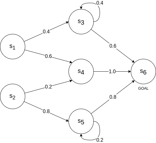
One way to solve this is via Dynamic Programming (DP). You can read more about it in my other blog post about Differential Dynamic Programming. What we need to know for now, though, is that we simply need to apply the Bellman Equation (Eq. 3) recursively to all states going from left to right:
\[\begin{aligned} V(s_6) &= 0 && \text{terminal state} \\ V(s_5) &= -1 + p(s_6 | s_5)V(s_6) + p(s_5|s_5)V(s_5) \\ &= -1 + 0.8 \cdot 0 + 0.2 V(s_5) \\ &= \dfrac{-1}{0.8} = -1.25 \\ V(s_4) &= -1 + 1.0 V(s_6) = -1 \\ V(s_3) &= -1 + 0.6 V(s_6) + 0.4 V(s_3) \\ &= -1 + 0.6 \cdot 0 + 0.4 V(s_3) \\ &= \dfrac{-1}{0.6} = -1 \dfrac{2}{3} \\ V(s_2) &= -1 + 0.2 V(s_4) + 0.8 V(s_5) \\ &= -1 -0.2 -0.8 \cdot 1.25 = -2.2 \\ V(s_1) &= -1 +0.4 V(s_3) + 0.6 V(s_4) \\ &= -1 -0.4 \cdot 1\dfrac{2}{3} - 0.6 \approx -2.2667 \end{aligned}\]Thus, by following the path of highest values, we can conclude that the best path is $s_2 \rightarrow s_4 \rightarrow s_6$. This is the power of value functions and how they allow us to estimate optimality and make decisions (well, in this example, we don’t actually decide).
We say that Dynamic Programming (DP):
- does full backups as it considers all possible transitions in Eq. 3. This works only for small problems.
- bootstraps as it uses other value estimates to update its own new estimates.
If we don’t want to bootstrap, we can instead use Monte Carlo (MC) samples to update our value estimates based on the full return of some sampled trajectories. In other words, we take multiple samples of Eq. 3 and use them to update our $V(s)$ estimates for all visited states $s$.
The full return in our toy example involves reaching the last termination state. We call this an episode.
There are multiple ways to MC estimates. The easiest one is first-visit MC, where we use the return following the first visit.
Using the same toy graph as above, say we are given 4 episodes:
- $s_1 \rightarrow s_3 \rightarrow s_3 \rightarrow s_6$
- results in $V(s_1) = -3$, $V(s_3)=-2$, $V(s_6)=0$
- $s_2 \rightarrow s_4 \rightarrow s_6$
- results in $V(s_2) = -2$, $V(s_4) = -1$, $V(s_6) = 0$
- $s_2 \rightarrow s_5 \rightarrow s_6$
- results in $V(s_2) = -2$, $V(s_5) = -1$, $V(s_6) = 0$
- $s_2 \rightarrow s_5 \rightarrow s_5 \rightarrow s_6$
- results in $V(s_2) = -3$, $V(s_5) = -2$, $V(s_6) = 0$
If we average out all the samples we get:
\[\begin{aligned} V(s_6) &= (0 + 0 + 0 + 0)/4 = 0 \\ V(s_5) &= (-1 - 2)/2 = -1.5 \\ V(s_4) &= -1 / 1= -1 \\ V(s_3) &= -2/1 = -2 \\ V(s_2) &= (-2 -2 -3)/3 = -2 \dfrac{1}{3} \\ V(s_1) &= -3/1 = -3 \end{aligned}\]Comparing these values to what we obtained in DP, we can see that they aren’t entirely correct but are close. If we have infinite MC samples, we will get the DP results according to the Weak Law of Large Numbers (WLLN). However, even with these 4 samples, we can still conclude that $s_2 \rightarrow s_4 \rightarrow s_6$ is the optimal path.
What is quite cool about MC is that we don’t need a model (i.e. it is model-free)! The not-so-cool thing is that we need to wait for episodes to finish before we can update our value estimates.
If we don’t want to wait until the end, we can use 1-step MC samples and bootstrap the rest:
\[V(s_t) \leftarrow V(s_t) + \alpha(\hat{V}(s_{t}) - V(s_t))\]where $\alpha$ is an update step and $\hat{V}(s_t)$ is our new estiamte for $V(s_t)$ (that we’re not fully certain of; that’s why we call it estimate). OK, but how can we get an estimate? We can use the definition of the value function from Eq. 2, but we must wait for the episode’s outcome. In Eq. 3, we discovered an interesting recursive relationship that only considers one step in the future. Swapping in that, we get a new update rule:
\[\begin{equation} V(s_t) \leftarrow V(s_t) + \alpha \bigg( \mathbb{E}_{a_t \sim \pi (a_t | s_t; \theta)} \bigg[ r(s_t, a_t) + \mathbb{E}_{s_{t+1} \sim p(s_{t+1} | s_{t})} \big[ V (s_{t+1}) \big] \bigg] - V(s_t) \bigg) \end{equation}\]Thus, now we have an update rule that we just need to wait for 1 timestep before applying! Note that we removed all remnants of $\pi$ and $a_t$ since we aren’t executing actions in this toy example.
This is called Temporal Difference (TD) Learning, and because we use only a single-step sample, this particular update is called a TD(0) update. This is a cross between DP and MC trying to harness the benefits of both. We can frequently update our estimates like DP by bootstrapping but also do so in a model-free fashion like MC!
TD-Learning is considered by many the core of RL! Armed with Eq. 6, we can conceive a simple value estimator algorithm for our toy problem.
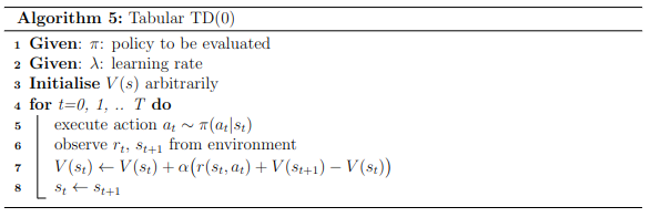
Let’s apply this to our toy problem. Initialise $V(s) = 0 \ \ \forall s$, $\alpha = 0.5$.
- $s_1 \rightarrow s_3 \rightarrow s_3 \rightarrow s_6$
- $V(s_1) = V(s_1) + 0.5(-1+V(s_3)-V(s_1)) = -0.5$
- $V(s_3) = V(s_3) + 0.5(-1+V(s_3)-V(s_3)) = -0.5$
- $V(s_3) = V(s_3) + 0.5(-1+V(s_6)-V(s_3)) = -0.75$
- $V(s_6) = V(s_6) = 0$
- $s_2 \rightarrow s_4 \rightarrow s_6$
- $V(s_2) = V(s_2) + 0.5(-1 + V(s_4) - V(s_2)) = -0.5$
- $V(s_4) = V(s_4) + 0.5(-1 + V(s_6) - V(s_4)) = -0.5$
- $V(s_6) = V(s_6) = 0$
- $s_2 \rightarrow s_5 \rightarrow s_6$
- $V(s_2) = V(s_2) + 0.5(-1 + V(s_5) - V(s_2)) = -0.75$
- $V(s_5) = V(s_5) + 0.5(-1 + V(s_6) - V(s_5)) = -0.5$
- $V(s_6) = V(s_6) = 0$
- $s_2 \rightarrow s_5 \rightarrow s_5 \rightarrow s_6$
- $V(s_2) = V(s_2) + 0.5(-1 + V(s_5) - V(s_2)) = -1.125$
- $V(s_5) = V(s_5) + 0.5(-1 + V(s_5) - V(s_5)) = -1$
- $V(s_5) = V(s_5) + 0.5(-1 + V(s_6) - V(s_5)) = -1$
- $V(s_6) = V(s_6) = 0$
Oh wow, we got the almost optimal path again! Let’s compare all of our value estimates from the different methods
| DP | MC | TD(0) | |
|---|---|---|---|
| $V(s_1)$ | 2.667 | -3 | -0.5 |
| $V(s_2)$ | -2.2 | -2.333 | -1.125 |
| $V(s_3)$ | -1.667 | -1.0 | -0.75 |
| $V(s_4)$ | -1.0 | -1.0 | -0.5 |
| $V(s_5)$ | -1.25 | -1.5 | -1.0 |
| $V(s_6)$ | 0.0 | 0.0 | 0.0 |
TD(0) didn’t do too badly! With more samples and more tuned $\alpha$ it can do even better! (Hint: try $\alpha=0.8$)
Going beyond TD(0)
TD(0) is a 1-step method, meaning that it waits for 1 step to rollout and then updates. There is extended and more general formulation of Temporal Difference Learning called TD($\lambda$) which can seamlessly take into account 0-step to infinite-step rollouts. This isn't necessary for deriving SAC but if you are intersted [Alister Reis has an interesting blog post](https://amreis.github.io/ml/reinf-learn/2017/11/02/reinforcement-learning-eligibility-traces.html) about it!
Q-Learning
TD-Learning is nice, but in the toy example above, we didn’t have a policy and thus an opportunity to take action. If we had the option, could we use TD-Learning to learn a policy?
One way is to take our TD(0) update from Eq. 6 and reformulate it with state-action values instead:
\[\begin{equation} Q(s_t, a_t) \leftarrow Q(s_t, a_t) + \alpha( r(s_t, a_t) + \mathbb{E}_{s_{t+1} \sim p(s_{t+1} | s_{t}, a_t) \atop a_t \sim \pi (a_t | s_t; \theta)} \big[ Q (s_{t+1}, a_{t+1}) \big] - Q(s_t, a_t)) \end{equation}\]OK, how do we select actions? The most naive way is by iterating over all actions to find the one with the highest value. Assuming a discrete and finite action space $A = \mathbb{N}^m$, then it is feasible to compute this.
\[a_t = \max_a Q(s_t, a)\]Let’s for a moment say we can feasibly compute this, then why should we compute the expected value of $Q(s_{t+1}, a_{t+1})$ in Eq. 7, why don’t we directly optimize Q there, which is guaranteed to lead to the optimal Q-value? Wait, what is the optimal Q-value?
Definition 3: The optimal value function $V^*(s)$ or $Q^*(s,a)$ is the value of following the optimal policy $\pi^*$ that achieves the highest possible reward on our task: $\forall s \in S, \forall \pi \neq \pi^*$ the following inequality holds $V^*(s) \geq V^\pi(s)$
Thus we can now reformulate Eq. 7 to always follow the (currently) optimal action, not just blindly use the sampled action:
\[\begin{equation} Q(s_t, a_t) \leftarrow Q(s_t, a_t) + \lambda( r(s_t, a_t) + \mathbb{E}_{s_{t+1} \sim p(s_{t+1} | s_{t}, a_t)} \big[ \max_a Q (s_{t+1}, a) \big] - Q(s_t, a_t)) \end{equation}\]For completeness and references to other literature, using Eq. 6 to update value estimates is known as SARSA, and using Eq. 8 is known as Q-Learning. Both are forms of TD-Learning. These two update rules represent on-policy and off-policy learning, respectively, which are two different schools in the RL community. On-policy updates have nice theoretical guarantees and, in practice, result in faster convergence but require us to learn from the current policy interacting with the environment. In contrast, off-policy approaches allow us to learn from any data and have better exploration but worse theoretical convergence guarantees.
OK, let’s get to something practical - how do we use Q-learning to solve interesting tasks?

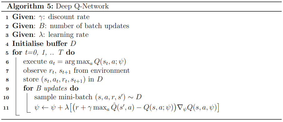
When Q is parameterised with a neural net, we arrive at the first successful deep RL algorithm - Deep Q-Network (DQN). In that paper, the authors parameterise the Q-value neural net with some parameters $\psi$ and train it to the loss function
\[\min_\psi \dfrac{1}{2} \big( r(s_t, a_t) + \gamma \max_a \hat{Q}(s_{t+1}, a) - Q(s_t, a_t; \psi) \big)^2\]which results in the update rule
\[\psi \leftarrow \psi + \lambda \big( r(s_t, a_t) + \gamma \max_a \hat{Q}(s_{t+1}, a) - Q(s_t, a_t; \psi) \big) \nabla_\psi Q(s_t, a_t; \psi)\]Okay, but where do we get the data to train on $(s_t, a_t, r_t, s_{t+1})$? With TD(0), we can learn from 1-step interactions, so we can do step, learn, step, learn and etc… However, NNs aren’t great at learning from a single data point; matter of fact, they only work when trained with Stochastic Gradient Descent (SGD). To make NNs work for Q-Learning, Mnih et al. introduce the concept of an experience replay buffer - a dataset containing the M latest interactions. If M is large enough (e.g. $10^6$), we can sample mini-batches from it and train our Q-network. Thus, we arrive at the famous DQN algorithm!
DQN details
OK, so I omitted some unimportant details regarding DQN:
1. What is $\gamma$? That is the discount rate, which we usually set to a number close to 1, like 0.99. We use it to discount the value of future rewards when we add it to the objective like $\sum_{t=0}^T \gamma^t r_t.
2. What is $\hat{Q}$? That is a "target network", which is a copy of our normal Q-network except that we don't backpropagate through it and that its parameters are lagging behind the main network by a few updates.
3. DQN also uses $\epsilon$-greedy exploration, where the robot takes a random action for each timestep with some probability. This is solely for adding naive exploration into the algorithm.
4. DQN also has the concept of a terminal value where instead of trying to minimise towards a target $r_t + \gamma \hat{Q}(s_t, a_t)$, we instead say that the episode terminates and we only minimise towards target $r_t$.
For all the details check the [original paper](https://arxiv.org/pdf/1312.5602)!
Policy Gradients
Q-learning is cool and works for deterministic action spaces, but let us now return to continuous action spaces $a_t \in A = R^d$. Finding $\max_a Q(s_t, a)$ becomes infeasibile. Even worse, as we increase $d$, we quickly run into the curse of dimensionality.
Let’s completely disregard Q-learning and return to having a parameterised policy $\pi(a, s; \theta)$ and optimise it to try to solve our base objective from Eq. 1. We can explicitly frame this as
\[\begin{equation} \max_{\theta} J(\theta) = \max_\theta \mathbb{E}_{s_{t+1} \sim p(s_{t+1} | s_{t}, a_{t}) \atop a_t \sim \pi(a_t | s_t; \theta)} \bigg[ \sum_{t=0}^T r(s_t, a_t) \bigg] \end{equation}\]Theorem 1: Policy Gradients (for finite horizon)
If our starting state follows some distribution $p(s_0)$, the gradient of the objective in Eq. 9 is
\[\begin{equation} \nabla_\theta J(\theta) = \mathbb{E}_{s_{t+1} \sim p(s_{t+1} | s_{t}, a_{t}) \atop a_t \sim \pi(a_t | s_t; \theta)} \bigg[ \sum_{t=0}^T r(s_t, a_t) \nabla_\theta \log \pi (a_t | s_t; \theta) \bigg] \end{equation}\]Pretty cool eh? This tells us that to optimize our objective, we don’t need to differentiate neither the reward, nor the model! This keeps up with our initial assumptions that we have no information about them.
Proof:
The key to the proof is the log-prob trick using the simple calculus identity
\[\nabla_x log f(x) = \dfrac{1}{f(x)} \nabla_x f(x)\] \[\nabla_x f(x) = f(x) \nabla_x \log f(x)\]If we apply this directly to Eq. 9 we get
\[\begin{equation} \nabla_\theta J (\theta) = J(\theta) \nabla_\theta \log J (\theta) \end{equation}\]Now, this is useful only if finding $\nabla_\theta \log J(\theta)$ is easy. Let’s check that
\[\begin{aligned} J(\theta) &= \max_\theta \mathbb{E}_{s_{t+1} \sim p(s_{t} | s_{t-1}, a_{t-1}) \atop a_t \sim \pi(a_t | s_t; \theta)} \bigg[ \sum_{t=0}^T r(s_t, a_t) \bigg]\\ &= \bigg[ \sum_{t=0}^T r(s_t, a_t) \bigg] \bigg[ \int_{s_0} p(s_0) \int_{a_0} \pi(a_0 | s_0; \theta) \int_{s_1} p(s_1|s_0, a_0) \int_{a_1} \pi (a_1 | s_1; \theta) \int_{s_2} p(s_2|s_1, a_1) ... \bigg] \\ &= \underbrace{\bigg[ \sum_{t=0}^T r(s_t, a_t) \bigg]}_\text{trajectory sample} \underbrace{\bigg[ \int_{s_0} p(s_0) \prod_{t=0}^T \int_{s_t} p(s_t| s_{t-1}, a_{t-1}) \int_{a_t} \pi (a_t | s_t; \theta) \bigg]}_\text{probability of trajectory sample} \end{aligned}\]Where $p(s_0 | s_{-1}, a_{-1}) = 1$
Let’s now take the log of the whole expression above
\[\log J(\theta) = \log \sum_{t=0}^T r(s_t, a_t) + \log \int_{s_0} p(s_0) + \sum_{t=0}^T \big[ \log \int_{s_t} p(s_t| s_{t-1}, a_{t-1}) + \log \int_{a_t} \pi(a_t|s_t; \theta) \big]\]Now taking the gradient of the whole expression, we see that most terms go away as they aren’t a function of $\theta$
\[\begin{aligned} \nabla \log J(\theta) &= \nabla_\theta \sum_{t=0}^T \log \int_{a_t} \pi (a_t|s_t; \theta) \\ &= \mathbb{E}_{s_{t+1} \sim p(s_{t+1} | s_{t}, a_{t}) \atop a_t \sim \pi(a_t | s_t; \theta)} \bigg[ \sum_{t=0}^T \nabla_\theta \log \pi(a_t|s_t; \theta) \bigg] \end{aligned}\]Plugging this directly into Eq. 11
\[\begin{aligned} \nabla_\theta J(\theta) &= J(\theta) \nabla_\theta \log J(\theta) \\ &= \mathbb{E}_{s_{t+1} \sim p(s_{t+1} | s_{t}, a_{t}) \atop a_t \sim \pi(a_t | s_t; \theta)} \bigg[\sum_{t=0}^T r(s_t, a_t) \bigg] \mathbb{E}_{s_{t+1} \sim p(s_{t+1} | s_{t}, a_{t}) \atop a_t \sim \pi(a_t | s_t; \theta)} \bigg[ \sum_{t=0}^T \nabla_\theta \log \pi(a_t | s_t; \theta) \bigg] \\ &= \mathbb{E}_{s_{t+1} \sim p(s_{t+1} | s_{t}, a_{t}) \atop a_t \sim \pi(a_t | s_t; \theta)} \bigg[ \sum_{t=0}^T r(s_t, a_t) \nabla_\theta \log \pi (a_t| s_t; \theta) \bigg] \end{aligned}\]Credits: I pieced together this proof from Sutton’s Chapter 13 and Tedrake’s Chapter 20.
Note: There are many other flavours of proofs for this theorem. One that is interesting to figure out is the infinite time horizon one.
We just developed this theory of optimising our objective; what now? Can we apply it to our problems and solve them? Kind of… The easiest approach we can derive is the Reinforce algorithm (Sutton 1999).
Assuming a finite-horizon problem, we can estimate take episodic Monte-Carlo samples of episode returns (objective Eq. 9) and use our Policy Gradients theorem to optimise some parametarised policy $\pi_\theta(a_t | s_t)$. To ease notation, we define a return sample as: $R_t = \sum_{i=t}^T r(s_i, a_i)$. Then the Reinforce algorithm is as follows
- Collect episode {$s_0, a_0, r_0, …, r_{T-1}, s$} following policy $\pi_\theta(\cdot | s_t)$
- For $ t = 0, …, T$
- $\theta \leftarrow \theta + \alpha R_t \nabla_\theta \log \pi_\theta (a_t | s_t)$
Reinforce is quite powerful but also inconviniently (and inefficiently) requires us to wait for an episode to finish before we can update our policy. This is especially bad when we are dealing with infinite horizon problems where $T = \infty$. Policy gradients (PG) methods are very useful, but they can’t figure out the long-term results of their actions - i.e. we just optimised to state $s_T$ but is that a good state to be in? It may be in the short term, but it may not be in the long term. I love giving the example of the drunken spider who had too much beer at the pub and is now trying to get home.
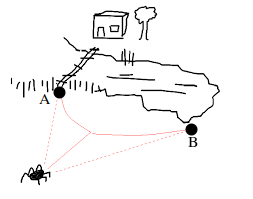
He is drunk, so his movement is uncertain (i.e. stochastic), and his planning horizon is severely limited. As a matter of fact, he is so drunk that he can only plan as much as points A and B. If we leave the spider to decide based on PG with a simple reward like the closest distance to home, it will decide that point A is better. However, then the spider has to cross the bridge, and if he stumbles, he will fall into the lake, which has a pretty bad reward. Thus, getting to state B is better, but PG needs more foresight to decide this due to their limited time horizon.
Actor critic methods
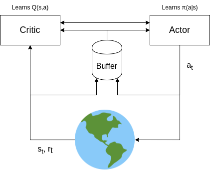
In a nutshell, actor-critic methods address the limitations of PG (lack of foresight) and Q-learning (inability to scale to continuous action spaces) by combining both ideas into one uniform framework called actor-critic methods. In a nutshell, they have three major components:
- A $\psi$-parametarised critic that lears a $Q(s,a; \psi)$ state-action value estimator based on Q-learning. We use our standard Eq. 8 but now we get our optimal action from $a_t \sim \pi(a_t | s_t; \theta)$. Thus our loss and update equations are now:
- A $\theta$-parametarised actor which learns according to our PG theorem Eq. 10. The key here is that instead of optimizing for maximal reward, we can optimize for the surrogate of the reward, the Q-function!
- Just like DQN, as we are using NNs here, it is a good idea to have an experience replay buffer and train both the actor and the critic back to back with sampled mini-batches and SGD.
Putting all these 3 blocks together we arrive at another famous algorithm called Deep Determinisitc Policy Gradients (DDPG) first presented by Lillicrap et al. in 2015
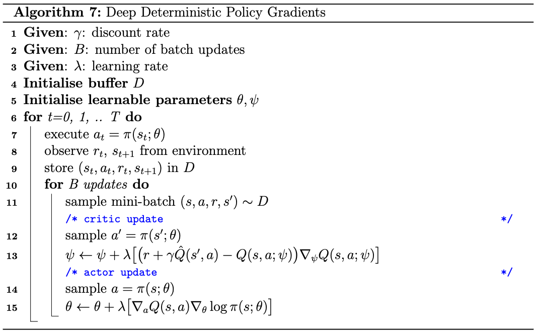
DDPG is pretty cool as it can now bring all the benefits of Q-learning into continuous action spaces, and it was the first method to successfully do more complex locomotion tasks. For the purposes of this blog post, we will investigate the (half-)cheetah and humanoid tasks of the Deepmind control suite:
Brief details about the tasks
* The half-cheetah has an observation space of 17 consisting of joint positions and angular velocities, as well as x, z positions Action space is torque over the 6 joints. Reward is forward velocity. * The humanoid has an observation space of 67, again consisting of positions, joint angles and angular velocities. The action space is 21 joint torque commands. The reward is reaching a velocity of 10 m/s.DDPG does quite well to the cheetah task but not so well on the humnoid one. Now (finally) we get to the main ordeal…
Soft Actor Critic
DDPG works well with some tricks added in, but it tends to be unstable and lacks exploration. This results in a tendency to get stuck in local minima without solving the task.
To alleviate this, Haarnoja et al. suggest we go back to using stochastic policies (unlike DDPG) and view the problem through the lens of entropy maximisation. For this, we look at entropy.
Definition 4: The entropy of a random variable $X$ designates the information value of $X$:
\[H(X) = \mathbb{E}[-\log p(X)] = - \int p(x) \log p(x)\]The intuition here is that less probable samples have a higher value(i.e. entropy) than more probable ones. Let’s say we have a distribution:
\[X = \begin{cases} a \quad \quad p=0.95 \\ b \quad \quad p=0.05 \end{cases}\]Computing the entropy, we get that $X=b$ has higher entropy:
\[H(X=a) = -p(X=a) \log p(X=a) \approx -0.05 \\ H(X=b) = -p(X=b) \log p(X=b) \approx -0.15\]That’s the intuition for a single sample, but the intuition for the entropy of the RV itself is counter intuitive. It measures how random a random variable is! In other words, how well distributed it is. Let’s look at two examples
\[H(X) = H(X=a) + H(X=b) \approx -0.2\] \[Y = \begin{cases} c \quad \quad p=0.5 \\ d \quad \quad p=0.5 \end{cases} \\ H(Y) = H(Y=c) + H(Y=d) \approx -0.69\]Cool, what now?
Entropy enables us to open another school of ideas: Maximum Entropy Reinforcement Learning (MaxEnt RL). In this line of work we redefine our initial objective in Eq. 1 as
\[\begin{equation} \max_\theta J(\theta) := \max_\theta \sum_{t=0}^T \mathbb{E}_{s_{t+1} \sim p(s_{t} | s_t, a_t) \atop a_t \sim \pi(a_t | s_t; \theta)} \big[ r(s_t, a_t) + \alpha H(\pi(a_t | s_t; \theta)) \big] \end{equation}\]where $\alpha$ is just a weighing coefficient (called temperature). In English, this reads as maximise the reward while being as random as possible. Somewhat counterintuitive, but this allows us to explore more efficiently and thus find a solution to the task. A new $J(\theta)$ means we also get new value functions:
\[\begin{equation} V^\pi(s_t) := \sum_{n=t}^T \mathbb{E}_{s_{n+1} \sim p(s_{n} | s_{n-1}, a_{n-1}) \atop a_n \sim \pi(a_n | s_n; \theta)} \big[ r(s_n, a_n) + \alpha H(\pi(a_t|s_t; \theta)) \big] \end{equation}\]$V^\pi(s_t)$ is nice but remeber that we need to decide on actions, so a state-action value is more useful:
\[\begin{align} Q^\pi(s_t, a_t) &:= r(s_t, a_t) + \mathbb{E}_{s_{t+1} \sim p(s_{t+1} | s_t, a_t)} [V^\pi (s_{t+1})] \\ & \text{Plug in Eq. 10} \notag \\ &= r(s_t,a_t) + \mathbb{E}_{s_{t+1} \sim p(s_{t+1} | s_t, a_t)} \bigg[ \sum_{n=t+1}^T \mathbb{E}_{s_{n+1} \sim p(s_{n+1}|s_n, a_n) \atop a_n \sim \pi(a_n| s_n; \theta)} \big[ r(s_n, a_n) -\alpha \log \pi(a_t | s_t; \theta) \big] \bigg] \notag \\ &\text{Note that $Q$ doesn't directly depend on $H(\cdot)$} \notag \\ &= r(s_t, a_t) + \mathbb{E}_{s_{t+1} \sim p(s_{t+1} | s_t, a_t) \atop a_{t+1} \sim \pi (a_{t+1} | s_{t+1}; \theta)} \bigg[ r(s_{t+1}, a_{t+1}) - \alpha \log \pi(a_{t+1}| s_{t+1}; \theta) + \sum_{n=t+2}^T \mathbb{E}_{s_{n+1} \sim p(s_{n+1}|s_n, a_n) \atop a_n \sim \pi(a_n| s_n; \theta)} \big[ r(s_n, a_n) -\alpha \log \pi(a_t | s_t; \theta) \big] \bigg] \notag \\ &= r(s_t, a_t) + \mathbb{E}_{s_{t+1} \sim p(s_{t+1} | s_t, a_t) \atop a_{t+1} \sim \pi (a_{t+1} | s_{t+1}; \theta)} \bigg[ r(s_{t+1}, a_{t+1}) - \alpha \log \pi(a_{t+1}| s_{t+1}; \theta) + \mathbb{E}_{s_{t+2} \sim p(s_{t+2}|s_{t+1}, a_{t+1})} [V^\pi(s_{t+2})] \bigg] \notag \\ &= r(s_t, a_t) + \mathbb{E}_{s_{t+1} \sim p(s_{t+1} | s_t, a_t) \atop a_{t+1} \sim \pi (a_{t+1} | s_{t+1}; \theta)} \bigg[ Q^\pi(s_{t+1}, a_{t+1}) - \alpha \log \pi(a_{t+1}| s_{t+1}; \theta)) \bigg] \end{align}\]We get the last line by plugging in Eq. 14. This is An interesting result! The Q function recursive relationship is different from the standard one we see in Q-learning (Eq. 5). The result in Eq. 16 is so important that it has a name: Soft Q-function. Inevitably this would lead us to Soft Actor Critic. First, let’s finish the critic part. With Eq. 16 and a $Q(s_t, a_t; \psi)$ parameterised by a neural net, we can formulate a new regression target and update it with SGD, just like we did in DQN:
\[\min_\psi \dfrac{1}{2} \big( r(s_t, a_t) + \gamma \mathbb{E}_{a_t \sim \pi(a_{t+1} | s_{t+1}; \theta)} [\hat{Q}(s_{t+1}, a_{t+1}) - \alpha \log \pi(a_{t+1| s_{t+1}; \theta})] - Q(s_t, a_t; \psi) \big)^2\]which results in the update rule
\[\psi \leftarrow \psi + \alpha \big( r(s_t, a_t) + \gamma \mathbb{E}_{a_t \sim \pi(a_{t+1} | s_{t+1}; \theta)} [\hat{Q}(s_{t+1}, a_{t+1}) - \alpha \log \pi(a_{t+1| s_{t+1}; \theta})] - Q(s_t, a_t; \psi) \big) \nabla_\psi Q(s_t, a_t; \psi)\]That handles the critic; now, how do we learn a policy? Since our policy is stochastic, that is non-trivial. I’m not sure how this part was derived in the SAC paper, but to me, it looks reverse engineered (please email me if you have a better clue!).
Our fundamental goal is to maximise the objective in Eq. 12. It’s clear to see that can be translated to something in terms of the Q-function:
\[\begin{aligned} \max_\theta J(\theta) &= \max_\theta \sum_{t=0}^T \mathbb{E}_{s_{t+1} \sim p(s_{t+1} | s_t, a_t) \atop a_{t} \sim \pi (a_{t} | s_{t}; \theta)} \big[ r(s_t, a_t) - \alpha \log \pi (a_t | s_t; \theta)] \\ &= \max_\theta \mathbb{E}_{a_0 \sim \pi (a_0|s_0;\theta)} \bigg[ r(s_0, a_0) - \alpha \log \pi(a_0|s_0;\theta) + \sum_{t=1}^T \mathbb{E}_{s_{t+1} \sim p(s_{t+1} | s_t, a_t) \atop a_{t} \sim \pi (a_{t} | s_{t}; \theta)} \big[ r(s_t, a_t) - \alpha \log \pi (a_t | s_t; \theta) \big] \bigg] \\ &= \max_\theta \mathbb{E}_{a_0 \sim \pi (a_0|s_0;\theta)} \bigg[ Q(s_1, a_1) - \alpha \log \pi(a_1|s_1; \theta) \bigg] \end{aligned}\]Thus we’d expect the gradient to be something proportional to $\log \pi (a | s;\theta) - Q(s, a)$, but unfortunately, we can’t just differentiate when $\pi$ is stochastic. We can be smarter with stochastic calculus and use the KL divergence:
\[\min_\theta D_{KL} \bigg( \pi(a_t |s_t; \theta) \ || \ \dfrac{\exp(Q^\pi(s_t, a_t))}{Z(s_t)} \bigg)\]My weak intuition
I read this as finding a distribution $pi$ that matches the distribution of $exp(Q^\pi(s, a))$. Why match? Because we want to be as random as possible. Why the exponent? because it makes the math later nice and doesn't change our objective. Why $Z(s_t)$? because distributions need to integrate to 1, and we can't guarantee that $Q(s_t,a_t)$ does. Drop me an email if you have a better idea!Using the definition of KL divergence we can expand this:
\[\begin{aligned} \min_\theta &D_{KL} \bigg( \pi(a_t |s_t; \theta) \ || \ \exp \big( Q(s_t,a_t) - \log Z(s_t) \big) \bigg) \\ &= \min_\theta - \int_{a_t} \pi(a_t|s_t;\theta) \log \bigg( \dfrac{\exp(Q(s_t, a_t) - \log Z(s_t))}{\pi(a_t|s_t;\theta)} \bigg) \\ &=\min_\theta -\int_{a_t} \pi (a_t|s_t;\theta) \big( \log \exp (Q(s_t, a_t) - \log Z(s_t)) - \log \pi (a_t | s_t; \theta) \big) \\ &=\min_\theta -\int_{a_t} \pi (a_t|s_t;\theta) \big( Q(s_t, a_t) - \log Z(s_t) - \log \pi (a_t | s_t; \theta) \big) \\ &= \min_\theta \mathbb{E}_{a_t \sim \pi(a_t|s_t;\theta)} \big[ \log Z(s_t) + \log \pi(a_t|s_t;\theta) - Q(s_t,a_t) \big] \end{aligned}\]Sampling data from a replay buffer, we can again optimize this with SGD:
\[\theta \leftarrow \theta + \lambda \big[ \alpha \nabla_\theta \log \pi(a_t|s_t;\theta) - \nabla_{a_t}Q(s_t, a_t) \nabla_\theta \log \pi (a_t|s_t;\theta) \big]\]This update equation looks nice, but $\nabla_\theta \pi$ isn’t straightforward. To make this tractable, we can restrict the policy to a set of well-known distributions like Gaussians. Then to make this backpropagatable, we can employ the reparametarization trick. If se set our policy to a diagonal Gaussian $\pi(a_t |s_t;\theta) = \mathcal{N}(\mu_\theta, \sigma_\theta)$, we can reparametarise it with a unit diagonal Gaussian as $\pi(a_t | s_t;\theta) = \mu_\theta + \sigma_\theta^T \mathcal{N}(0, 1)$.
With this, we can now complete our first basic SAC algorithm:
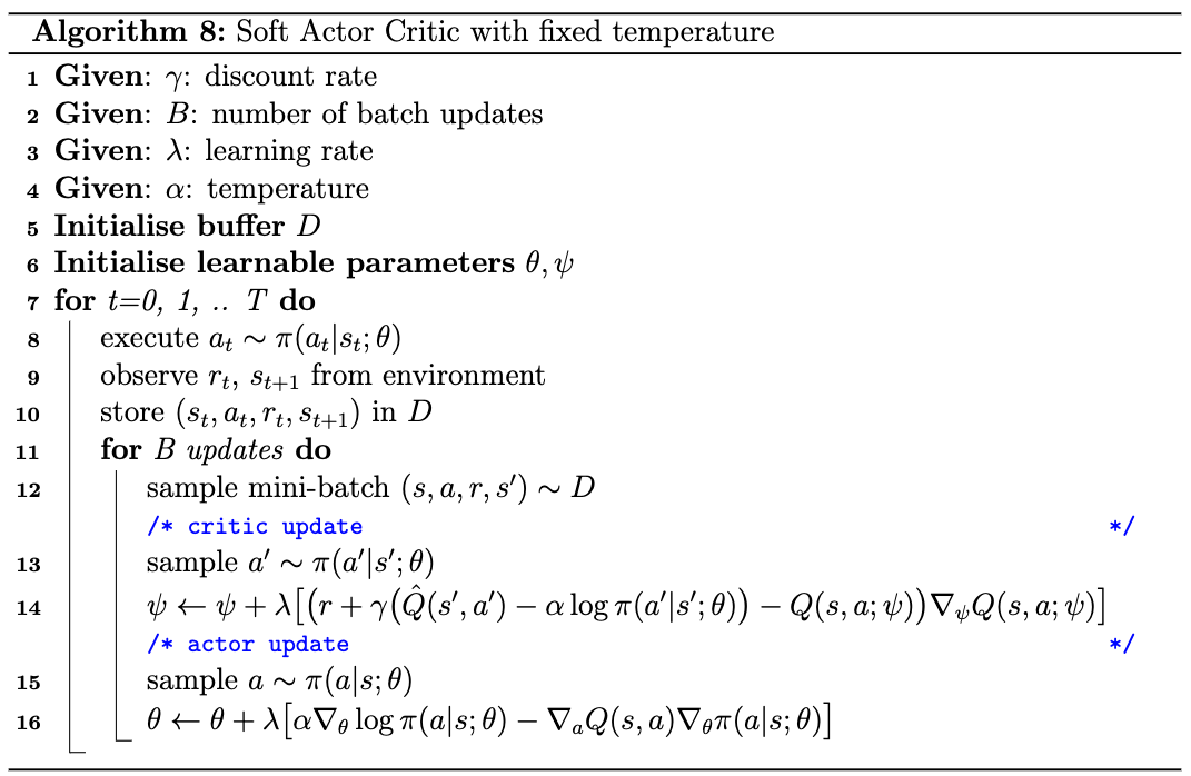
When applied to the cheetah problem, SAC does well but can’t even match DDPG in terms of both training or evaluation.
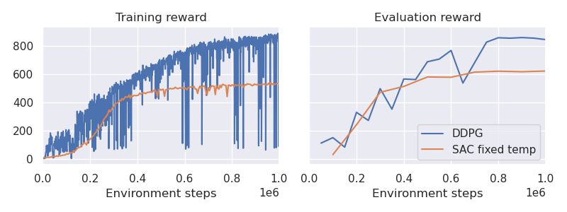
SAC does well initially and is more stable than DDPG, but as we approach the optimal policy, performance starts getting worse. The issue is that fixed-temperature SAC has one major limitation, as the name implies - the $\alpha$ parameter is fixed! This means that during training, we care equally about exploration. This is why SAC matches DDPG at the early stages of training but later starts lagging behind.
Naturally, though, we want to explore the early stages of training. Once we’ve done some exploration, we want to prioritise solving the task (i.e. maximising the reward) as efficiently as possible. The straightforward to achieve this would be to decrease $\alpha \rightarrow 0$ over time. That would probably work, but remember that we’re using stochastic policies. They can tell us how confident they are about their actions! Thus we can use the confidence of the policy itself to adjust $\alpha$ automatically!
Soft Actor Critic with automatic temperature
In their 2018 paper, Haarnoja et al. extend SAC to automatically adjust its entropy temperature $\alpha$ by targeting a minimum entropy level.
They do this by reframing the maximum entropy RL objective in Eq. 12 to maintain a minimum entropy level at all times instead of explicitly maximising entropy. Mathematically this translates to the constrained objective
\[\max_\theta \mathbb{E}_{s_{t+1} \sim p(s_{t+1}|s_t,a_t) \atop a_t \sim \pi (a_t| s_t; \theta)} \big[ \sum_{t=0}^T r(s_t, a_t) \big] \\ s.t. \quad \mathbb{E}_{s_{t+1} \sim p(s_{t+1}|s_t,a_t) \atop a_t \sim \pi (a_t| s_t; \theta)} \big[ -\log \pi(a_t | s_t; \theta) \big] \geq H_0\]Where $H_0$ is the minimum entropy we are trying to maintain. This constraint makes things more difficult to optimise. One way to do that is via the method of Lagrange multipliers. To apply that, we need to reshuffle our constraint in the form of $-H_0 - \mathbb{E} \big[\ log \pi (a_t | s_t; \theta) \big] \geq 0$. Then we can form our Lagrangian at the last timestep $T$ as follow below:
\[\begin{aligned} \mathcal{L}(\theta_T, \alpha_T) &= \mathbb{E}_{s_{t+1} \sim p(s_{t+1}|s_t,a_t) \atop a_t \sim \pi (a_t| s_t; \theta_T)} [r(s_T, a_T)] - \alpha_T \big( H_0 + \mathbb{E}_{s_{t+1} \sim p(s_{t+1}|s_t,a_t) \atop a_t \sim \pi (a_t| s_t; \theta_T)} [\log \pi(a_t | s_T; \theta_T)] \big) \\ &= \mathbb{E}_{s_{t+1} \sim p(s_{t+1}|s_t,a_t) \atop a_t \sim \pi (a_t| s_t; \theta_T)} \big[ r(s_T, a_T) - \alpha_T H_0 - \alpha_T \log \pi(a_T|s_T; \theta_T) \big] \end{aligned}\]Note: for this proof, we will be iterating backwards through the trajectory and finding the optimal parameters for each step. This means we have policy parameters $\theta_T$ and $\alpha_T$ that are optimal for the objective function at timestep $T$.
Assuming strong duality (i.e. that the optimal policy that solves the task has entropy $\geq H_0$), we can establish that solving our objective yields the same solution as solving our Lagrangian as:
\[\max_{\theta_T} J(\theta_T) = \min_{\alpha_T \geq 0} \max_{\pi_T} \mathcal{L}(\theta_T, \alpha_T)\]Due to the assumed strong duality, we know that the optimal temperature would be:
\[\begin{align} \alpha^*_T &= \text{argmin}_{\alpha_T \geq 0} \max_{\theta_T} \mathcal{L}(\theta_T, \alpha_T) \notag \\ &= \text{argmin}_{\alpha_T \geq 0} \max_{\theta_T} \mathbb{E}_{s_{t+1} \sim p(s_{t+1}|s_t,a_t) \atop a_t \sim \pi_T (a_t| s_t; \theta_T)} \big[ r(s_T, a_T) - \alpha_T H_0 - \alpha_T \log \pi(a_T|s_T; \theta_T) \big] \end{align}\]Here we see a 2-step optimisation problem: first, we solve for $\pi$, then we solve for $\alpha$. Thus we can also view the above equation as:
\[\alpha^*_T = \text{argmin}_{\alpha_T \geq 0} \mathbb{E}_{s_{t+1} \sim p(s_{t+1}|s_t,a_t) \atop a_t \sim \pi (a_t| s_t; \theta_T^*)} \big[ r(s_T, a_T) - \alpha_T H_0 - \alpha_T \log \pi(a_T|s_T; \theta_T^*) \big]\]OK, we have an expression for solving $\alpha_T$ but what about $t=0,1,\ …\ ,T-1$? Let’s go back through time using the soft-Q relationship that we previously established in Eq. 15 in order to find $\pi_{T-1}^*$:
\[\begin{aligned} \max_{\theta_{T-1}} &\mathbb{E}_{a_{T-1} \sim \pi(a_{T-1}|s_{T-1}; \theta_{T-1})} [r(s_{T-1}, a_{T-1}) + \max_{a_T} r(s_T, a_T)] \\ & \text{By rearanging our soft-Q from Eq.16 we can} \\ &= \max_{\theta_{T-1}} Q(s_{T-1}, a_{T-1}) - \alpha_T H_0 \\ &\text{Since this is the primal, we can equate it to the dual} \\ &= \min_{\alpha_{T-1}} \max_{\theta_{T-1}} \mathbb{E}_{s_{T-1} \sim p(s_{T-1}|s_{T-2},a_{T-2}) \atop a_{T-1} \sim \pi (a_{T-1}| s_{T-1}; \theta_{T-1})} \bigg[ Q^*_{T-1} (s_{T-1}, a_{T-1}) - \alpha_{T-1}H_0 - \alpha_{T-1} \log \pi (a_{T-1}|s_{T-1}; \theta_{T-1}) \bigg] - \alpha_T H_0 \end{aligned}\]By applying this recursively down to $t=0$ we get the generic $\alpha$ loss function:
\[\min_{\alpha} \mathbb{E}_{a_t \sim \pi^*(a_t|s_t;\theta)} \big[ -\alpha \log \pi^* (a_t | s_t; \theta) - \alpha H_0 \big]\]Note: The SAC paper also features a derivation of the infinite-time version of SAC, but this blog post is concerned only with finite-time problems. That being said, I can’t understand the continuous time proof/derivation in the appendix of the paper.
Since we are now trying to solve our objective via the Lagrangian, we must constantly alternate between solving for $\theta$ and solving for $\alpha$ until convergence. However, SAC is an actor-critic method; thus, we also need to alternate between optimising for the critic parameters $\psi$. The critic here is optimised just like before. Adding that into the mix, we get to the complete SAC algorithm:
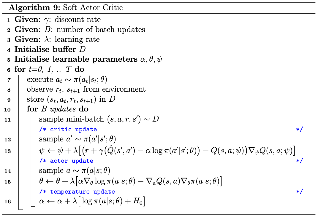
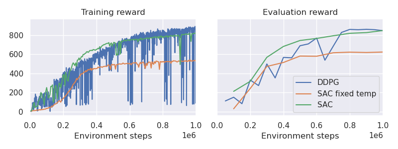
OK, so how does it perform against other algorithms? SAC outperforms DDPG across the board now. Returning to our cheetah and humanoid examples:
Cheetah
Humanoid
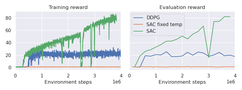
We can now see that SAC is not only outperforming DDPG but is also significantly more stable! On a very practical note, SAC is also easier to tune when setting up different problems. I was too lazy to leave SAC run until convergence on the humanoid task, but here are some more extensive results on all DMC tasks.
Refernces
- Reinforcement Learning: An Introduction by Sutton and Barto
- Underactuated robotics by Russ Tedrake
- Deep Deterministic Policy Gradients, Lillicrap et al. (2015)
- SAC papertrail:
Further resources
- denisyarats/pytorch_sac. A good high-performant SAC implementation.
- Lilian Weng’s blog post about policy gradients. She covers most approaches that use the theorem. Recommended!
Acknowledgements
Krishnan Srinivasan for bouncing off ideas and listening to me ramble about this
If you have any comments or suggestions, shoot me an email!