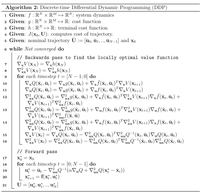
Differential Dynamic Programming (DDP), first proposed by David Mayne in 1965 is one of the oldest trajectory optimization techniques in optimal control literature. It is an extension of Dynamic Programming where instead of optimising over the full state space, we are only optimise around a nominal trajectory by taking 2nd order Taylor approximations. Doing this repeatedly allows us to find local solutions of non-linear trajectory optimisation problems. Although simple in principle, it is a surprisingly powerful method which was more recently re-discovered and simplified into iLQR by Tassa et al and showcased in complex humanoid behaviour.
In this blog post I’ll go over the theory and derivation behind DDP which goes along nicely with my implementation of it found on GitHub.
Table of contents
- The optimal control problem
- Dynamic Programming (DP)
- Differential Dynamic Programming (DDP)
- Implementation details
- Experimental result
The optimal control problem
Given a continuous-time system with state $\textbf{x}\in \mathbb{R}^N$ and control $\textbf{u}\in \mathbb{R}^M$ characterised by the dynamics:
\[\begin{aligned} % \label{eq:dynamics} \dfrac{d\textbf{x}}{dt} = f(\textbf{x}(t), \textbf{u}(t), t)\end{aligned}\]we want to minimise the cost function:
\[\begin{aligned} % \label{eq:cost-func} J(\textbf{x}(t_0), \pi) = \underbrace{h(\textbf{x}(t_f), t_f)}_{\text{terminal cost}} + \int_{t_0}^{t_f} \underbrace{g(\textbf{x}(t), \textbf{u}(t), t)}_{\text{cost-to-go}} dt\end{aligned}\]This can be read as the cumulative cost of following a policy $\pi$ starting at state $\textbf{x}(t_0)$. Our goal now is to find the optimal policy $\pi^*$ which finds the minimal cost:
\[\begin{aligned} % \label{eq:optimal-control-problem} \pi^* = \arg \min_\pi J(\textbf{x}(t_0), \pi)\end{aligned}\]Assuming time-invariant dynamics, this problem can also be discretised as follows. Given a fixed time horizon $N$, define our timestep $\Delta t = \dfrac{t_f - t_0}{N}$
\[\begin{aligned} % \label{eq:discrete-dynamics} \dfrac{\textbf{x}(t_k + \Delta t) - \textbf{x}(t_k)}{\Delta t} & \approx f(\textbf{x}(t_k), \textbf{u}(t_k)) \\ \textbf{x}(t_k + \Delta t_k) & = \textbf{x}(t_k) + \Delta t f(\textbf{x}(t_k), \textbf{u}(t_k)) \\ \textbf{x}(t_{k+1}) & = \textbf{x}(t_k) + \Delta t f(\textbf{x}(t_k), \textbf{u}(t_k)) \\ \textbf{x}_{k+1} & = \textbf{x}_k + \Delta t f(\textbf{x}_k, \textbf{u}_k)\end{aligned}\]where in the final line we make the notational simplification $\textbf{x}_k := \textbf{x}(t_k)$ for convenience and ease of reading. This will become cumbersome to navigate around later.
In a similar fashion, we can also discretise the cost function to:
\[\begin{aligned} J(\textbf{x}_0, \pi) = h(\textbf{x}_N, t_N) + \sum_{k=0}^{N-1} g(\textbf{x}_k, \textbf{u}_k, t_k)\end{aligned}\]For the remainder of this we will assume that both our cost function are time-invariant:
\[\begin{aligned} % \label{eq:discrete-cost} J(\textbf{x}_0, \pi) = h(\textbf{x}_N) + \sum_{k=0}^{N-1} g(\textbf{x}_k, \textbf{u}_k)\end{aligned}\]Dynamic Programming (DP)
The approach that is neither dynamic nor involves programming. Thanks Dr Bellman!
Let us think about a discrete graph which we want to traverse from the start node to the goal node with minimal cost as in Figure below. Think of each node as a state $\textbf{x}$ with a value $V(\textbf{x})$ which designates the remaining cost of reaching the goal from this state. Each outgoing edge from a node can be taught of as a discrete action with an associated cost-to-go $g(\textbf{x}, \textbf{u})$ and naturally the goal state will have a terminal cost $h(\textbf{x}_{\text{goal}})=0$.
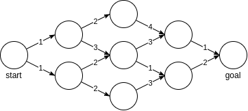
One way to find the optimal path through the graph is via the Bellman optimality principle which states that the optimal value of a state is the lowest combination of cost-to-go and the value of the subsequent state $\textbf{x}’$:
\[\begin{aligned} V^*(\textbf{x}) = \min_\textbf{u}[ g(\textbf{x}, \textbf{u}) + V^*(\textbf{x}') ]\end{aligned}\]If we have some magic oracle to give us the optimal value of $\textbf{x}’$ then this formulation allows us to go backwards in time and compute the optimal value of every $\textbf{x}$. Luckily, for our toy problem (and beyond), we already have the optimal value of the final state as there are no decisions to be made:
\[\begin{aligned} V^*(\textbf{x}_{\text{goal}}) = \min_\textbf{u}[ h(\textbf{x}_{\text{goal}}) ] = \min_\textbf{u}[0] = 0\end{aligned}\]Now continuing backwards in time, using Bellman equation, we can estimate the value of every state
Once we have the value of each node/state, we can easily find the path of lowest cost by simply looking to the next reachable states and choosing the one with the lowest cost. Matter of fact, we can do this from any node we want, not just the start node. Now let us be more rigorous, what is the definition of a value $V(\textbf{x})$? It is the cost we will incur if we start from $\textbf{x}$ and try to reach the goal. Previously we saw the optimal value $V^*(\textbf{x})$ which gives us the best-case cost. However, a more general formulation is the value under some policy $\pi$ which might be optimal or might not be, it doesn’t matter:
\[\begin{aligned} % \label{eq:bellman-discrete} V^\pi(\textbf{x}_n, t_n) & = \min_\textbf{u}\bigg[ J(\textbf{x}_n, \pi) \bigg] = \min_\textbf{u}\bigg[ \sum_{k=n}^{N-1} g(\textbf{x}_k, \textbf{u}_k) + h(\textbf{x}_N) \bigg] \\ & = \min_\textbf{u}\bigg[ g(\textbf{x}_n, \textbf{u}_n) + \underbrace{\sum_{k=n+1}^{N-1} g(\textbf{x}_k, \textbf{u}_k) + h(\textbf{x}_N)}_{V^\pi(\textbf{x}_{n+1}, n+1)} \bigg] \\ & = \min_\textbf{u}\bigg[ g(\textbf{x}_n, \textbf{u}_n) + V^\pi (\textbf{x}_{n+1}, n+1) \bigg]\end{aligned}\]where $\textbf{x}_{n+1} = f(\textbf{x}_n, \textbf{u}_n)$. This recursive relationship is known as the discrete Bellman Equation.
Using this we can now create an algorithm for solving problems as in the figures above by going backwards in time:
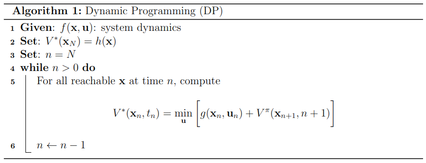
DP is great in theory and works well for very small problems but it has one big issue - it suffers from the curse of dimensionality. If we have say $>10^8$ reachable $\textbf{x}_n$ at line 5 of the algorithm, then computation becomes intractable. This becomes an even bigger issue when we’re dealing with continuous systems.
One way to deal with the curse of dimensionality is with Differential Dynamic Programming (DDP).
Differential Dynamic Programming (DDP)
Instead of computing the values over the entire state space via DP, we can be smarter by only computing the values around our best-guess trajectory and iteratively closing in on the actual optimal solution. We do this optimisation iteratively by linearising the dynamics and cost around our current trajectory and taking 2nd order steps towards the optimal solution as shown in the figure below:
![DDP applied to an inverted
pendulum problem. The pendulum is initialised at a stationary downwards
facing position $[\theta, \dot{\theta}] = [\pi, 0]$ and we want to reach
a stationary upwards facing position $[\theta, \dot{\theta}] = [0, 0]$.
The plot visualises how DDP takes iterative steps towards the optimal
trajectory by locally linearising the
cost.](/img/blog/2023-02-01-ddp/ddp_optimizations_low_steps.png "fig:")
In addition to the discrete time-invariant dynamics and cost, we now also define a fixed-horizon control sequence which in turn defines our trajectory (state sequence).
\[\begin{aligned} \text{given }\textbf{x}_0, \textbf{U} := [\textbf{u}_0, \textbf{u}_1, .. , \textbf{u}_{N-1}] \implies \textbf{X} := [\textbf{x}_1, \textbf{x}_2, .. , \textbf{x}_{N}]\end{aligned}\]Then our optimal control problem can be redefined as
\[\begin{aligned} \textbf{U}^* &= \arg \min_{\textbf{U}} J(\textbf{x}_0, \textbf{U}) \\ &= \arg \min_{\textbf{U}} \left[ h(\textbf{x}_N) + \sum_{n=0}^{N-1} g(\textbf{x}_n, \textbf{u}_n) \right]\end{aligned}\]where the subsequent states are given by our dynamics. As with most problems spanning from the curse of dimensionality, a good way to solve it would be to do some form of approximation. Assuming we have a starting trajectory, a good way to do a local approximation would be to do a Taylor series expansion.
Taylor series expansion
Doing a Taylor series expansion around a function is a way of approximating to an arbitrary degree. We often use this to convert difficult to solve and interpret functions into convex ones that we know how to solve. Given a function $f: \mathbb{R}^N \mapsto \mathbb{R}$ and $\textbf{x}\in \mathbb{R}^N$ an infinite Taylor series expansion around some arbitrary point $\bar{\textbf{x}}$ is given by
\[\begin{aligned} f(\textbf{x}) = f(\bar{\textbf{x}}) + \dfrac{1}{1!} \sum_{i=1}^{N} \dfrac{\partial f(\textbf{x})}{\partial x_i} \Bigr\rvert_{\textbf{x}=\bar{\textbf{x}}} (x_i - \bar{x}_i) + \dfrac{1}{2!} \sum_{i=1}^{N} \dfrac{\partial^2 f(\textbf{x})}{\partial x_i^2} \Bigr\rvert_{\textbf{x}=\bar{\textbf{x}}} (x_i - \bar{x}_i)^2 + ...\end{aligned}\]To make the derivation easier to follow we will adopt the notation $\dfrac{\partial f(\textbf{x})}{\partial x_i} \Bigr\rvert_{\textbf{x}=\bar{\textbf{x}}} := \dfrac{\partial f(\bar{\textbf{x}})}{\partial x_i}$, thus we can rewrite the Taylor series expansion into a more compact form:
\[\begin{aligned} f(\textbf{x}) = f(\bar{\textbf{x}}) + \dfrac{1}{1!} \sum_{i=1}^{N} \dfrac{\partial f(\bar{\textbf{x}})}{\partial x_i} (x_i - \bar{x}_i) + \dfrac{1}{2!} \sum_{i=1}^{N} \dfrac{\partial^2 f(\bar{\textbf{x}})}{\partial x_i^2} (x_i - \bar{x}_i)^2 + ...\end{aligned}\]The summation is correct but difficult to work with. We can rewrite it in terms of the gradient $\nabla f(\textbf{x})$
\[\begin{aligned} \sum_{i=1}^{N} \dfrac{\partial f(\bar{\textbf{x}})}{\partial x_i} (x_i - \bar{x}_i) = \begin{bmatrix} \dfrac{\partial f(\bar{\textbf{x}})}{\partial x_1} \\[10pt] \dfrac{\partial f(\bar{\textbf{x}})}{\partial x_2} \\[10pt] \vdots \\[10pt] \dfrac{\partial f(\bar{\textbf{x}})}{\partial x_N} \\ \end{bmatrix}^T \begin{bmatrix} x_1 - \bar{x}_1 \\ x_2 - \bar{x}_2 \\ \vdots \\ x_N - \bar{x}_N \\ \end{bmatrix} = \nabla f(\bar{\textbf{x}})^T (\textbf{x}- \bar{\textbf{x}}) \end{aligned}\]Which now allows us to write the Taylor expansion in a more elegant form:
\[\begin{aligned} % \label{eq:taylor_series} f(\textbf{x}) &= f(\bar{\textbf{x}}) + \dfrac{1}{1!} \nabla f(\textbf{x})^T (\textbf{x}- \bar{\textbf{x}}) + \dfrac{1}{2!} \nabla^2 f(\textbf{x})^T (\textbf{x}- \bar{\textbf{x}})^2 + ... \\ &= \sum_{n=0}^{R=\infty} \dfrac{1}{n!} \nabla^n f(\textbf{x})^T (\textbf{x}- \bar{\textbf{x}})^n\end{aligned}\]Here is a neat visualisation of Taloy Series approximations:
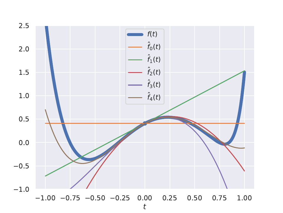
Note: To do Taylor series approximation our function must be continuous and infinitely differentiable. Some functions such as sinusoids satisfy this property, but for most functions we only approximate to the R-th order which requires the function to be only R times differentiable.
For the purposes of DDP (and optimisation as a whole), we are interested in 2nd order approximations due to their inherent convexity. Thus for the remainder of this we will focus on 2nd order approximations. When dealing with dynamical systems, functions are usually in the format we defined before. As such, we need to extend the function we defined above to $f: \mathbb{R}^N \mapsto \mathbb{R}^N$. What does this mean for $\nabla f(\textbf{x})$ as used in the Taylor series? We now need to differentiate every dimensions of $f(\textbf{x})$ with respect to every individual $x_i$. That transforms our gradient to a Jacobian of the format:
\[\begin{aligned} \nabla f(\bar{\textbf{x}}) = \begin{bmatrix} \dfrac{\partial f_1(\bar{\textbf{x}})}{\partial x_1} & \dfrac{\partial f_2(\bar{\textbf{x}})}{\partial x_1} & \dots & \dfrac{\partial f_N(\bar{\textbf{x}})}{\partial x_1} \\[10pt] \dfrac{\partial f_1(\bar{\textbf{x}})}{\partial x_2} & \dfrac{\partial f_2(\bar{\textbf{x}})}{\partial x_2} & \dots & \dfrac{\partial f_N(\bar{\textbf{x}})}{\partial x_2} \\[10pt] \vdots & & \ddots & \vdots \\[10pt] \dfrac{\partial f_1(\bar{\textbf{x}})}{\partial x_N} & \dots & \dots & \dfrac{\partial f_N(\bar{\textbf{x}})}{\partial x_N} \\[10pt] \end{bmatrix}\end{aligned}\]The final modification we need to make to turn f into a standard dynamic equation is to add the control input $\textbf{u}\in \mathbb{R}^M$ as a variable of f, which transforms it to $f: \mathbb{R}^N \times \mathbb{R}^M \mapsto \mathbb{R}^N$. Since $f$ is now a function of two variables, we need to introduce additional notation $\nabla_\textbf{x}f(\bar{\textbf{x}}, \bar{\textbf{u}})$ for taking the Jacobian (or gradient) with respect to $\textbf{x}$ and evaluating it at $(\bar{\textbf{x}}, \bar{\textbf{u}})$. Armed with this we can now do a 2nd order Taylor series approximation:
\[\begin{aligned} f(\textbf{x}, \textbf{u}) \approx& f(\bar{\textbf{x}}, \bar{\textbf{u}}) + \nabla_\textbf{x}f(\bar{\textbf{x}}, \bar{\textbf{u}})^T (\textbf{x}- \bar{\textbf{x}}) + \nabla_\textbf{u}f(\bar{\textbf{x}}, \bar{\textbf{u}})^T (\textbf{u}- \bar{\textbf{u}}) + \\ & \dfrac{1}{2}(\textbf{x}- \bar{\textbf{x}})^T \nabla_\textbf{xx}^2 f(\bar{\textbf{x}}, \bar{\textbf{u}})^T (\textbf{x}- \bar{\textbf{x}}) + \dfrac{1}{2}(\textbf{u}- \bar{\textbf{u}})^T \nabla_\textbf{ux}^2 f(\bar{\textbf{x}}, \bar{\textbf{u}})^T (\textbf{x}- \bar{\textbf{x}}) + \\ & \dfrac{1}{2}(\textbf{x}- \bar{\textbf{x}})^T \nabla_\textbf{xu}^2 f(\bar{\textbf{x}}, \bar{\textbf{u}})^T (\textbf{u}- \bar{\textbf{u}}) + \dfrac{1}{2}(\textbf{u}- \bar{\textbf{u}})^T \nabla_\textbf{uu}^2 f(\bar{\textbf{x}}, \bar{\textbf{u}})^T (\textbf{u}- \bar{\textbf{u}}) \\ =& f(\bar{\textbf{x}}, \bar{\textbf{u}}) + \begin{bmatrix} \nabla_\textbf{x}f(\bar{\textbf{x}}, \bar{\textbf{u}})\\ \nabla_\textbf{u}f(\bar{\textbf{x}}, \bar{\textbf{u}}) \end{bmatrix}^T \begin{bmatrix} \textbf{x}- \bar{\textbf{x}}\\ \textbf{u}- \bar{\textbf{u}} \end{bmatrix} + \dfrac{1}{2} \begin{bmatrix} \textbf{x}- \bar{\textbf{x}}\\ \textbf{u}- \bar{\textbf{u}} \end{bmatrix}^T \begin{bmatrix} \nabla_\textbf{xx}^2 f(\bar{\textbf{x}}, \bar{\textbf{u}}) & \nabla_\textbf{xu}^2 f(\bar{\textbf{x}}, \bar{\textbf{u}})\\ \nabla_\textbf{ux}^2 f(\bar{\textbf{x}}, \bar{\textbf{u}}) & \nabla_\textbf{uu}^2 f(\bar{\textbf{x}}, \bar{\textbf{u}}) \end{bmatrix} \begin{bmatrix} \textbf{x}- \bar{\textbf{x}}\\ \textbf{u}- \bar{\textbf{u}} \end{bmatrix}\end{aligned}\]where the second equality is only rearranging terms in vector form for easier manipulation.
Since $f(\textbf{x}, \textbf{u})$ is the equation describing the dynamics of some system $\dot{\textbf{x}} = \dfrac{d\textbf{x}}{dt} = f(\textbf{x}, \textbf{u})$, we can rewrite the above approximation as
\[\begin{aligned} f(\textbf{x}, \textbf{u}) - f(\bar{\textbf{x}}, \bar{\textbf{u}}) \approx \begin{bmatrix} \nabla_\textbf{x}f(\bar{\textbf{x}}, \bar{\textbf{u}})\\ \nabla_\textbf{u}f(\bar{\textbf{x}}, \bar{\textbf{u}}) \end{bmatrix}^T \begin{bmatrix} \textbf{x}- \bar{\textbf{x}}\\ \textbf{u}- \bar{\textbf{u}} \end{bmatrix} + \dfrac{1}{2} \begin{bmatrix} \textbf{x}- \bar{\textbf{x}}\\ \textbf{u}- \bar{\textbf{u}} \end{bmatrix}^T \begin{bmatrix} \nabla_\textbf{xx}^2 f(\bar{\textbf{x}}, \bar{\textbf{u}}) & \nabla_\textbf{xu}^2 f(\bar{\textbf{x}}, \bar{\textbf{u}})\\ \nabla_\textbf{ux}^2 f(\bar{\textbf{x}}, \bar{\textbf{u}}) & \nabla_\textbf{uu}^2 f(\bar{\textbf{x}}, \bar{\textbf{u}}) \end{bmatrix} \begin{bmatrix} \textbf{x}- \bar{\textbf{x}}\\ \textbf{u}- \bar{\textbf{u}} \end{bmatrix} \\ \dfrac{d\textbf{x}}{dt} - \dfrac{d\bar{\textbf{x}}}{dt} \approx \begin{bmatrix} \nabla_\textbf{x}f(\bar{\textbf{x}}, \bar{\textbf{u}})\\ \nabla_\textbf{u}f(\bar{\textbf{x}}, \bar{\textbf{u}}) \end{bmatrix}^T \begin{bmatrix} \textbf{x}- \bar{\textbf{x}}\\ \textbf{u}- \bar{\textbf{u}} \end{bmatrix} + \dfrac{1}{2} \begin{bmatrix} \textbf{x}- \bar{\textbf{x}}\\ \textbf{u}- \bar{\textbf{u}} \end{bmatrix}^T \begin{bmatrix} \nabla_\textbf{xx}^2 f(\bar{\textbf{x}}, \bar{\textbf{u}}) & \nabla_\textbf{xu}^2 f(\bar{\textbf{x}}, \bar{\textbf{u}})\\ \nabla_\textbf{ux}^2 f(\bar{\textbf{x}}, \bar{\textbf{u}}) & \nabla_\textbf{uu}^2 f(\bar{\textbf{x}}, \bar{\textbf{u}}) \end{bmatrix} \begin{bmatrix} \textbf{x}- \bar{\textbf{x}}\\ \textbf{u}- \bar{\textbf{u}} \end{bmatrix} \\ % actual newline \dfrac{d(\textbf{x}- \bar{\textbf{x}})}{dt} \approx \begin{bmatrix} \nabla_\textbf{x}f(\bar{\textbf{x}}, \bar{\textbf{u}})\\ \nabla_\textbf{u}f(\bar{\textbf{x}}, \bar{\textbf{u}}) \end{bmatrix}^T \begin{bmatrix} \textbf{x}- \bar{\textbf{x}}\\ \textbf{u}- \bar{\textbf{u}} \end{bmatrix} + \dfrac{1}{2} \begin{bmatrix} \textbf{x}- \bar{\textbf{x}}\\ \textbf{u}- \bar{\textbf{u}} \end{bmatrix}^T \begin{bmatrix} \nabla_\textbf{xx}^2 f(\bar{\textbf{x}}, \bar{\textbf{u}}) & \nabla_\textbf{xu}^2 f(\bar{\textbf{x}}, \bar{\textbf{u}})\\ \nabla_\textbf{ux}^2 f(\bar{\textbf{x}}, \bar{\textbf{u}}) & \nabla_\textbf{uu}^2 f(\bar{\textbf{x}}, \bar{\textbf{u}}) \end{bmatrix} \begin{bmatrix} \textbf{x}- \bar{\textbf{x}}\\ \textbf{u}- \bar{\textbf{u}} \end{bmatrix}\end{aligned}\]where in the last line we use the linearity of the derivative operator. Finally to make notation even more compact, we introduce (yet another) pair of terms $\delta \textbf{x}= \textbf{x}- \bar{\textbf{x}}$ and $\delta \textbf{u}= \textbf{u}- \bar{\textbf{u}}$. These allows us to nicely rewrite the equation above to
\[\begin{aligned} % \label{eq:taylor-expansion} \dfrac{d\delta \textbf{x}}{dt} = f(\delta \textbf{x}, \delta \textbf{u}) \approx \begin{bmatrix} \nabla_\textbf{x}f(\bar{\textbf{x}}, \bar{\textbf{u}})\\ \nabla_\textbf{u}f(\bar{\textbf{x}}, \bar{\textbf{u}}) \end{bmatrix}^T \begin{bmatrix} \delta \textbf{x}\\ \delta \textbf{u} \end{bmatrix} + \dfrac{1}{2} \begin{bmatrix} \delta \textbf{x}\\ \delta \textbf{u} \end{bmatrix}^T \begin{bmatrix} \nabla_\textbf{xx}^2 f(\bar{\textbf{x}}, \bar{\textbf{u}}) & \nabla_\textbf{xu}^2 f(\bar{\textbf{x}}, \bar{\textbf{u}})\\ \nabla_\textbf{ux}^2 f(\bar{\textbf{x}}, \bar{\textbf{u}}) & \nabla_\textbf{uu}^2 f(\bar{\textbf{x}}, \bar{\textbf{u}}) \end{bmatrix} \begin{bmatrix} \delta \textbf{x}\\ \delta \textbf{u} \end{bmatrix}\end{aligned}\]Backwards pass
Armed with the Taylor series expansion, we can now return to the Bellman Equation and convert it to a local 2nd order approximation.
\[\begin{aligned} V(&\textbf{x}_n, t_n) = \min_{\textbf{u}} \bigg[ g(\textbf{x}_n, \textbf{u}_n) + V(\textbf{x}_{n+1}, t_{n+1}) \bigg] \\ &= \min_\textbf{u}\bigg[ g(\textbf{x}_n + \bar{\textbf{x}}_n - \bar{\textbf{x}}_n, \textbf{u}_n + \bar{\textbf{u}}_n - \bar{\textbf{u}}_n) + V(\textbf{x}_{n+1} + \bar{\textbf{x}}_{n+1} - \bar{\textbf{x}}_{n+1}, t_{n+1})) \bigg] \\ & \text{substitute with } \delta \textbf{x}_n := \textbf{x}_n - \bar{\textbf{x}}_n \text{ and } \delta \textbf{u}_n := \textbf{u}_n - \bar{\textbf{u}}_n \\ &= \min_{\delta \textbf{u}} \bigg[ g(\delta \textbf{x}_n + \bar{\textbf{x}}_n, \delta \textbf{u}_n + \bar{\textbf{u}}_n) + V(\delta \textbf{x}_{n+1} + \bar{\textbf{x}}_{n+1}, t_{n+1}) \bigg]\end{aligned}\]Now it’s time to do the Taylor series approximation according to how we defined it. That is straightforward for $g(\delta \textbf{x}_n + \bar{\textbf{x}}_n, \delta \textbf{u}_n + \bar{\textbf{u}}_n)$ since it is a simple function. However, $V(\delta \textbf{x}_{n+1} + \bar{\textbf{x}}_{n+1}, t_{n+1})$ is less straightforward as it depends on our dynamics $f$:
\[\begin{aligned} V(\delta \textbf{x}_{n+1} + &\bar{\textbf{x}}_{n+1}, t_{n+1}) \\ &\approx V(\bar{\textbf{x}}_{n+1}, t_{n+1}) + \nabla_\textbf{x}V(\bar{\textbf{x}}_{n+1}, t_{n+1}) \Bigr\rvert_{\textbf{x}=\bar{\textbf{x}}_{n+1}}^T \delta \textbf{x}_{n+1} + \delta \textbf{x}_{n+1}^T \nabla_\textbf{xx}^2 V(\bar{\textbf{x}}_{n+1}, t_{n+1}) \Bigr\rvert_{\textbf{x}=\bar{\textbf{x}}_{n+1}} \delta \textbf{x}_{n+1} \\ &= V(\bar{\textbf{x}}_{n+1}, t_{n+1}) \nabla_\textbf{x}V(\bar{\textbf{x}}_{n+1}, t_{n+1})^T \delta \textbf{x}_{n+1} + \delta \textbf{x}_{n+1}^T \nabla_\textbf{xx}^2 V(\bar{\textbf{x}}_{n+1}, t_{n+1}) \delta \textbf{x}_{n+1}\end{aligned}\]where as before we use the notation
\[\nabla_\textbf{x}V(\bar{\textbf{x}}_{n+1}, t_{n+1}) := \nabla_\textbf{x}V(\textbf{x}, t_{n+1}) \Bigr\rvert_{\textbf{x}=\bar{\textbf{x}}_{n+1}}\]Now we can do another approximation but this time of our dynamics in order to get to the bottom of the value function approximation above:
\[\begin{aligned} \dfrac{d\delta \textbf{x}}{dt} & = f(\delta \textbf{x}, \delta \textbf{u}) \approx \nabla_\textbf{x}f(\textbf{x}, \textbf{u})\Bigr\rvert_{\textbf{x}=\bar{\textbf{x}}, \textbf{u}=\bar{\textbf{u}}} \delta \textbf{x}+ \nabla_\textbf{u}f(\textbf{x}, \textbf{u})\Bigr\rvert_{\textbf{x}=\bar{\textbf{x}}, \textbf{u}=\bar{\textbf{u}}} \delta \textbf{u}\\ & = \nabla_\textbf{x}f (\bar{\textbf{x}}, \bar{\textbf{u}}) \delta \textbf{x}+ \nabla_\textbf{u}f (\bar{\textbf{x}}, \bar{\textbf{u}}) \delta \textbf{u}\\ \delta \textbf{x}_{n+1} - \delta \textbf{x}_n &\approx \nabla_\textbf{x}f (\bar{\textbf{x}}_n, \bar{\textbf{u}}_n) \delta \textbf{x}_n + \nabla_\textbf{u}f (\bar{\textbf{x}}_n, \bar{\textbf{u}}_n) \delta \textbf{u}_n \\ \delta \textbf{x}_{n+1} &\approx \delta \textbf{x}_n + \nabla_\textbf{x}f (\bar{\textbf{x}}_n, \bar{\textbf{u}}_n) \delta \textbf{x}_n + \nabla_\textbf{u}f (\bar{\textbf{x}}_n, \bar{\textbf{u}}_n) \delta \textbf{u}_n \\ & = (I + \nabla_\textbf{x}f (\bar{\textbf{x}}_n, \bar{\textbf{u}}_n))\delta \textbf{x}_n + \nabla_\textbf{u}f (\bar{\textbf{x}}_n, \bar{\textbf{u}}_n) \delta \textbf{u}_n \\ & = \nabla_\textbf{x}\tilde{f} (\bar{\textbf{x}}_n, \bar{\textbf{u}}_n) \delta \textbf{x}_n + \nabla_\textbf{u}f (\bar{\textbf{x}}_n, \bar{\textbf{u}}_n) \delta \textbf{u}_n\end{aligned}\]Now plug this back into our value function approximation:
\[\begin{aligned} V(\delta \textbf{x}_{n+1} + &\bar{\textbf{x}}_{n+1}, t_{n+1}) \approx V(\bar{\textbf{x}}_{n+1}, t_{n+1}) + \nabla_\textbf{x}V(\bar{\textbf{x}}_{n+1}, t_{n+1})^T \big(\nabla_\textbf{x}\tilde{f} \delta \textbf{x}_n + \nabla_\textbf{u}f \delta \textbf{u}_n\big) \\ & \hspace{1cm} + \big( \nabla_\textbf{x}\tilde{f} \delta \textbf{x}_n + \nabla_\textbf{u}f \delta \textbf{u}_n \big)^T \nabla_\textbf{xx}^2 V(\bar{\textbf{x}}_{n+1}, t_{n+1}) \big( \nabla_\textbf{x}\tilde{f} \delta \textbf{x}_n + \nabla_\textbf{u}f \delta \textbf{u}_n \big) \\ &= V(\bar{\textbf{x}}_{n+1}, t_{n+1}) + \nabla_\textbf{x}V(\bar{\textbf{x}}_{n+1}, t_{n+1})^T \nabla_\textbf{x}\tilde{f} \delta \textbf{x}_n + \nabla_\textbf{x}V(\bar{\textbf{x}}_{n+1}, t_{n+1})^T \nabla_\textbf{u}f \delta \textbf{u}_n \\ & \hspace{1cm} + \big( \delta \textbf{x}_n^T \nabla_\textbf{x}\tilde{f}^T \nabla_\textbf{xx}^2 V(\bar{\textbf{x}}_{n+1}, t_{n+1}) + \delta \textbf{u}_n^T \nabla_\textbf{u}f^T \nabla_\textbf{xx}^2 V(\bar{\textbf{x}}_{n+1}, t_{n+1}) \big) \big( \nabla_\textbf{x}\tilde{f} \delta \textbf{x}_n + \nabla_\textbf{u}f \delta \textbf{u}_n \big) \\ &= V(\bar{\textbf{x}}_{n+1}, t_{n+1}) + \nabla_\textbf{x}V(\bar{\textbf{x}}_{n+1}, t_{n+1})^T \nabla_\textbf{x}\tilde{f} \delta \textbf{x}_n + \nabla_\textbf{x}V(\bar{\textbf{x}}_{n+1}, t_{n+1})^T \nabla_\textbf{u}f \delta \textbf{u}_n \\ & \hspace{1cm} + \delta \textbf{x}_n^T \nabla_\textbf{x}\tilde{f}^T \nabla_\textbf{xx}^2 V(\bar{\textbf{x}}_{n+1}, t_{n+1}) \nabla_\textbf{x}\tilde{f} \delta \textbf{x}_n + \delta \textbf{x}_n^T \nabla_\textbf{x}\tilde{f}^T \nabla_\textbf{xx}^2 V(\bar{\textbf{x}}_{n+1}, t_{n+1}) \nabla_\textbf{u}f \delta \textbf{u}_n \\ & \hspace{1cm} + \delta \textbf{u}_n^T \nabla_\textbf{u}f^T \nabla_\textbf{xx}^2 V(\bar{\textbf{x}}_{n+1}, t_{n+1}) \nabla_\textbf{x}\tilde{f} \delta \textbf{x}_n + \delta \textbf{u}_n^T \nabla_\textbf{u}f^T \nabla_\textbf{xx}^2 V(\bar{\textbf{x}}_{n+1}, t_{n+1}) \nabla_\textbf{u}f \delta \textbf{u}_n\end{aligned}\]Combining this with the 2nd order expansion of $g$ we get an approximation of our Bellman Equation:
\[\begin{aligned} % \label{eq:value-func-taylor-approx} % \begin{split} % not supported by katex V(\textbf{x}_n, t_n) \approx \min_{\delta \textbf{u}_n} \big[ &g(\bar{\textbf{x}}_n, \bar{\textbf{u}}_n) + V(\bar{\textbf{x}}_{n+1}, t_{n+1}) \\ & + \big( \nabla_\textbf{x}g + \nabla_\textbf{x}\tilde{f}^T \nabla_\textbf{x}V(\bar{\textbf{x}}_{n+1}, t_{n+1}) \big)^T \delta \textbf{x}_n \\ & + \big( \nabla_\textbf{u}g(\bar{\textbf{x}}_n, \bar{\textbf{u}}_n) + \nabla_\textbf{u}f^T \nabla_\textbf{x}V(\bar{\textbf{x}}_{n+1}, t_{n+1}) \big)^T \delta \textbf{x}_n \\ & + \delta \textbf{x}_n^T \big( \nabla_\textbf{xx}^2 g(\bar{\textbf{x}}_n, \bar{\textbf{u}}_n) + \nabla_\textbf{x}\tilde{f}^T \nabla_\textbf{xx}^2 V(\bar{\textbf{x}}_{n+1}, t_{n+1}) \nabla_\textbf{x}\tilde{f} \big) \delta \textbf{x}_n \\ & + \delta \textbf{x}_n^T \big( \nabla_\textbf{xu}^2 g(\bar{\textbf{x}}_n, \bar{\textbf{u}}_n) + \nabla_\textbf{x}\tilde{f}^T \nabla_\textbf{xx}^2 V(\bar{\textbf{x}}_{n+1}, t_{n+1}) \nabla_\textbf{u}f \big) \delta \textbf{u}_n \\ & + \delta \textbf{u}_n^T \big( \nabla_\textbf{ux}^2 g(\bar{\textbf{x}}_n, \bar{\textbf{u}}_n) + \nabla_\textbf{u}f^T \nabla_\textbf{xx}^2 V(\bar{\textbf{x}}_{n+1}, t_{n+1}) \nabla_\textbf{x}\tilde{f} \big) \delta \textbf{x}_n \\ & + \delta \textbf{u}_n^T \big( \nabla_\textbf{uu}^2 g(\bar{\textbf{x}}_n, \bar{\textbf{u}}_n) + \nabla_\textbf{u}f^T \nabla_\textbf{xx}^2 V(\bar{\textbf{x}}_{n+1}, t_{n+1}) \nabla_\textbf{u}f \big) \delta \textbf{u}_n \big] % \end{split} % not supported by katex \end{aligned}\]Notice how all the terms inside the bracket are only derivatives. If we introduce a new helpful notation which is commonly referred to as the state-action value function $Q$:
\[\begin{aligned} % \label{eq:state-action-value} Q(\textbf{x}_n, \textbf{u}_n, t_n) = g(\textbf{x}_n, \textbf{u}_n) + V(\textbf{x}_{n+1}, t_{n+1})\end{aligned}\]we can re-express the value function as:
\[\begin{aligned} V(\textbf{x}_n, t_n) \approx \min_{\delta \textbf{u}_n} \big[ &Q(\bar{\textbf{x}}_n, \bar{\textbf{u}}_n, t_n) + \nabla_\textbf{x}Q(\bar{\textbf{x}}_n, \bar{\textbf{u}}_n, t_n) \delta \textbf{x}_n \\ & + \nabla_\textbf{u}Q(\bar{\textbf{x}}_n, \bar{\textbf{u}}_n, t_n) \delta \textbf{x}_n + \delta \textbf{x}_n^T \nabla_\textbf{xx}^2 Q(\bar{\textbf{x}}_n, \bar{\textbf{u}}_n, t_n) \delta \textbf{x}_n \\ & + \delta \textbf{x}_n^T \nabla_\textbf{xu}^2 Q(\bar{\textbf{x}}_n, \bar{\textbf{u}}_n, t_n) \delta \textbf{u}_n + \delta \textbf{u}_n^T \nabla_\textbf{ux}^2 Q(\bar{\textbf{x}}_n, \bar{\textbf{u}}_n, t_n) \delta \textbf{x}_n \\ & + \delta \textbf{u}_n^T \nabla_\textbf{uu}^2 Q(\bar{\textbf{x}}_n, \bar{\textbf{u}}_n, t_n) \delta \textbf{u}_n \big]\end{aligned}\]This resembles a (strange) Taylor series approximation! Well actually, this is exactly a Taylor series approximation around $Q(\bar{\textbf{x}}_n, \bar{\textbf{u}}_n, t_n)$! We can even rewrite our Bellman Equation as:
\[\begin{aligned} % \label{eq:bellman-approx-with-q} % \begin{split} % not supported by katex V(\textbf{x}_n, t_n) &= \min_{\delta \textbf{u}_n} \big[ g(\textbf{x}_n, \textbf{u}_n) + V(\textbf{x}_{n+1}, t_{n+1}) \big] \\ & = \min_{\delta \textbf{u}_n} \big[ Q(\textbf{x}_n, \textbf{u}_n, t_n) \big] \\ & \approx \min_{\delta \textbf{u}_n} \big[ Q(\bar{\textbf{x}}_n, \bar{\textbf{u}}_n, t_n) + Q(\delta \textbf{x}_n, \delta \textbf{u}_n, t_n) \big] \\ & = \min_{\delta \textbf{u}_n} \big[ Q(\delta \textbf{x}_n, \delta \textbf{u}_n, t_n) \big] + Q(\bar{\textbf{x}}_n, \bar{\textbf{u}}_n, t_n) % \end{split} % not supported by katex \end{aligned}\]where
\[\begin{aligned} % \label{eq:ddp-q} Q(\delta \textbf{x}_n, \delta \textbf{u}_n, t_n) \approx& \begin{bmatrix} \nabla_\textbf{x}Q(\bar{\textbf{x}}_n, \bar{\textbf{u}}_n, t_n)\\ \nabla_\textbf{u}Q(\bar{\textbf{x}}_n, \bar{\textbf{u}}_n, t_n) \end{bmatrix}^T \begin{bmatrix} \delta \textbf{x}_n \\ \delta \textbf{u}_n \end{bmatrix} + \dfrac{1}{2} \begin{bmatrix} \delta \textbf{x}_n \\ \delta \textbf{u}_n \end{bmatrix}^T \begin{bmatrix} \nabla_\textbf{xx}^2 Q(\bar{\textbf{x}}_n, \bar{\textbf{u}}_n, t_n) & \nabla_\textbf{xu}^2 Q(\bar{\textbf{x}}_n, \bar{\textbf{u}}_n, t_n)\\ \nabla_\textbf{ux}^2 Q(\bar{\textbf{x}}_n, \bar{\textbf{u}}_n, t_n) & \nabla_\textbf{uu}^2 Q(\bar{\textbf{x}}_n, \bar{\textbf{u}}_n, t_n) \end{bmatrix} \begin{bmatrix} \delta \textbf{x}_n \\ \delta \textbf{u}_n \end{bmatrix}\end{aligned}\]where each $Q$ derivative can be extracted from our derivation before, however, this time we are doing a 2nd order approximation of the dynamics whereas before we did a 1st order approximation.
\[\begin{aligned} % \label{eq:ddp-derivatives} % \begin{split} % not supported by katex \nabla_\textbf{x}Q(\bar{\textbf{x}}_n, \bar{\textbf{u}}_n, t_n) &= \nabla_\textbf{x}g(\bar{\textbf{x}}_n, \bar{\textbf{u}}_n) + \nabla_\textbf{x}\tilde{f}^T \nabla_{\textbf{x}} V(\bar{\textbf{x}}_{n+1}, t_{n+1}) \\ \nabla_\textbf{u}Q(\bar{\textbf{x}}_n, \bar{\textbf{u}}_n, t_n) &= \nabla_\textbf{u}g(\bar{\textbf{x}}_n, \bar{\textbf{u}}_n) + \nabla_\textbf{u}f^T \nabla_{\textbf{x}} V(\bar{\textbf{x}}_{n+1}, t_{n+1}) \\ \nabla_\textbf{xx}^2 Q(\bar{\textbf{x}}_n, \bar{\textbf{u}}_n, t_n) &= \nabla_\textbf{xx}^2 g(\bar{\textbf{x}}_n, \bar{\textbf{u}}_n) + \nabla_\textbf{x}\tilde{f}^T \nabla_{\textbf{x}\textbf{x}}^2 V(\bar{\textbf{x}}_{n+1}, t_{n+1}) \nabla_\textbf{x}\tilde{f} + \nabla_{\textbf{x}} V(\bar{\textbf{x}}_{n+1}, t_{n+1})^T \nabla_\textbf{xx}^2 \tilde{f} \\ \nabla_\textbf{uu}^2 Q(\bar{\textbf{x}}_n, \bar{\textbf{u}}_n, t_n) &= \nabla_\textbf{uu}^2 g(\bar{\textbf{x}}_n, \bar{\textbf{u}}_n) + \nabla_\textbf{u}f^T \nabla_{\textbf{x}\textbf{x}}^2 V(\bar{\textbf{x}}_{n+1}, t_{n+1}) \nabla_\textbf{u}f + \nabla_{\textbf{x}} V(\bar{\textbf{x}}_{n+1}, t_{n+1})^T \nabla_\textbf{uu}^2 f \\ \nabla_\textbf{ux}^2 Q(\bar{\textbf{x}}_n, \bar{\textbf{u}}_n, t_n) &= \nabla_\textbf{ux}^2 g(\bar{\textbf{x}}_n, \bar{\textbf{u}}_n) + \nabla_\textbf{u}f^T \nabla_{\textbf{x}\textbf{x}}^2 V(\bar{\textbf{x}}_{n+1}, t_{n+1}) \nabla_\textbf{x}\tilde{f} + \nabla_{\textbf{x}} V(\bar{\textbf{x}}_{n+1}, t_{n+1})^T \nabla_\textbf{ux}^2 f % \end{split} % not supported by katex \end{aligned}\]Now that we have our clearly defined Taylor series approximation of $Q$, we can start solving the optimisation program. For the time being, we do drop time notation for time-dependency to make the derivation easier to follow:
\[\begin{aligned} % \label{eq:u*} &\delta \textbf{u}^* = \arg \min_{\delta \textbf{u}} Q(\delta \textbf{x}, \delta \textbf{u}) \\ &\nabla_{\delta \textbf{u}} Q(\delta \textbf{x}, \delta \textbf{u}) = \textbf{0} \\ &\nabla_{\delta \textbf{u}} \Bigg[ \begin{bmatrix} \nabla_\textbf{x}Q(\bar{\textbf{x}}, \bar{\textbf{u}})\\ \nabla_\textbf{u}Q(\bar{\textbf{x}}, \bar{\textbf{u}}) \end{bmatrix}^T \begin{bmatrix} \delta \textbf{x}\\ \delta \textbf{u} \end{bmatrix} + \dfrac{1}{2} \begin{bmatrix} \delta \textbf{x}\\ \delta \textbf{u} \end{bmatrix}^T \begin{bmatrix} \nabla_\textbf{xx}^2 Q(\bar{\textbf{x}}, \bar{\textbf{u}}) & \nabla_\textbf{xu}^2 Q(\bar{\textbf{x}}, \bar{\textbf{u}})\\ \nabla_\textbf{ux}^2 Q(\bar{\textbf{x}}, \bar{\textbf{u}}) & \nabla_\textbf{uu}^2 Q(\bar{\textbf{x}}, \bar{\textbf{u}}) \end{bmatrix} \begin{bmatrix} \delta \textbf{x}\\ \delta \textbf{u} \end{bmatrix} \Bigg] = \textbf{0} \\ &\nabla{\delta \textbf{u}} \bigg[ \nabla_\textbf{x}Q(\bar{\textbf{x}}, \bar{\textbf{u}})^T \delta \textbf{x}+ \nabla_\textbf{u}Q(\bar{\textbf{x}}, \bar{\textbf{u}})^T \delta \textbf{u}+ \dfrac{1}{2} \delta \textbf{x}^T \nabla_\textbf{xx}^2Q(\bar{\textbf{x}}, \bar{\textbf{u}}) \delta \textbf{x}+ \\ & \hspace{3cm} \dfrac{1}{2}\delta \textbf{u}^T \nabla_\textbf{ux}^2 Q(\bar{\textbf{x}}, \bar{\textbf{u}}) \delta \textbf{x}+ \dfrac{1}{2} \delta \textbf{x}^T \nabla_\textbf{xu}^2 Q(\bar{\textbf{x}}, \bar{\textbf{u}}) \delta \textbf{u}+ \dfrac{1}{2} \delta \textbf{u}^T \nabla_\textbf{uu}^2 Q(\bar{\textbf{x}}, \bar{\textbf{u}}) \delta \textbf{u}\bigg] = \textbf{0} \\ &\nabla{\delta \textbf{u}} \bigg[ \nabla_\textbf{x}Q(\bar{\textbf{x}}, \bar{\textbf{u}})^T \delta \textbf{x}+ \nabla_\textbf{u}Q(\bar{\textbf{x}}, \bar{\textbf{u}})^T \delta \textbf{u}+ \dfrac{1}{2} \delta \textbf{x}^T \nabla_\textbf{xx}^2Q(\bar{\textbf{x}}, \bar{\textbf{u}}) \delta \textbf{x}+ \\ & \hspace{3cm} \delta \textbf{u}^T \nabla_\textbf{ux}^2 Q(\bar{\textbf{x}}, \bar{\textbf{u}}) \delta \textbf{x}+ \dfrac{1}{2} \delta \textbf{u}^T \nabla_\textbf{uu}^2 Q(\bar{\textbf{x}}, \bar{\textbf{u}}) \delta \textbf{u}\bigg] = \textbf{0} \\ &\text{(using the property that Hessians are symmetrical)} \\ &\nabla_\textbf{u}Q(\bar{\textbf{x}}, \bar{\textbf{u}})^T + \delta \textbf{x}^T \nabla_\textbf{ux}^2 Q(\bar{\textbf{x}}, \bar{\textbf{u}})^T + \delta \textbf{u}^T \nabla_\textbf{uu}^2 (\bar{\textbf{x}}, \bar{\textbf{u}}) = \textbf{0} \\ &\text{(transposing)} \\ &\nabla_\textbf{u}Q(\bar{\textbf{x}}, \bar{\textbf{u}}) + \nabla_\textbf{ux}^2 Q(\bar{\textbf{x}}, \bar{\textbf{u}}) \delta \textbf{x}+ \nabla_\textbf{uu}^2 Q(\bar{\textbf{x}}, \bar{\textbf{u}}) \delta \textbf{u}= \textbf{0} \\ &\nabla_\textbf{uu}^2 Q(\bar{\textbf{x}}, \bar{\textbf{u}}) \delta \textbf{u}= -\nabla_\textbf{u}Q(\bar{\textbf{x}}, \bar{\textbf{u}}) - \nabla_\textbf{ux}^2 Q(\bar{\textbf{x}}, \bar{\textbf{u}}) \delta \textbf{x}\\ &\delta \textbf{u}^* = -\nabla_\textbf{uu}^2 Q(\bar{\textbf{x}}, \bar{\textbf{u}})^{-1} (\nabla_\textbf{u}Q(\bar{\textbf{x}}, \bar{\textbf{u}}) + \nabla_\textbf{ux}^2 Q(\bar{\textbf{x}}, \bar{\textbf{u}}) \delta \textbf{x}) \\ &\delta \textbf{u}^* = \underbrace{- \nabla_\textbf{uu}^2 Q(\bar{\textbf{x}}, \bar{\textbf{u}})^{-1} \nabla_\textbf{u}Q(\bar{\textbf{x}}, \bar{\textbf{u}})}_{\text{feed-forward term}} - \underbrace{\nabla_\textbf{uu}^2 Q^{-1}(\bar{\textbf{x}}, \bar{\textbf{u}}) \nabla_\textbf{ux}^2 Q(\bar{\textbf{x}}, \bar{\textbf{u}}) \delta \textbf{x}}_{\text{feedback term}}\end{aligned}\]Turns out that DDP not only gives us the optimal "motor tape" feed-forward control sequence but also gives us the optimal feedback similar to LQR but here we approximate 2nd order system dynamics!
Note: Solving for $\delta \textbf{u}$ is the same as optimising for $\textbf{u}$ as the $\bar{\textbf{u}}$ in $\delta \textbf{u}= \textbf{u}- \bar{\textbf{u}}$ is fixed.
Now that we have a closed-form expression for computing $\delta \textbf{u}^* $ , we can start using our time-variance again and optimize a trajectory! Starting at the end of the trajectory at timestep $t=N$ and going backwards in time where in each timestep, we approximate $Q(\delta \textbf{x}_n, \delta \textbf{u}_n, t_n)$ and use it to compute $\delta \textbf{u}^*_n$ via equation above. Rolled out this would give us the sequence $[\delta \textbf{u}^*_N, \delta \textbf{u}^*_{N-1}, .. ,\delta \textbf{u}^*_{0}]$ which seemingly gives us our locally optimal trajectory.
Notice that this has one fatal limitation - when computing our $\delta \textbf{u}^*_n$ we always use the approximation of the value function around the initial nominal state trajectory $\textbf{X} := [\textbf{x}_0, \textbf{x}_1, .. , \textbf{x}_N]$. This would (eventually) give us results but we can do better! Since we are changing the value functions using $\delta \textbf{u}^*_n$, we can also use it to estimate how our value function changes.
To get a more explicit expression for how we compute this we have to plug in the value of $\delta \textbf{u}^*$ into the 2nd order approximation of $Q$ and we get:
\[\begin{aligned} &V(\textbf{x}, t_n) = Q(\delta \textbf{x}, \delta \textbf{u}^*, t_n) + Q(\bar{\textbf{x}}, \bar{\textbf{u}}, t_n) \\ &= \nabla_\textbf{x}Q(\bar{\textbf{x}}, \bar{\textbf{u}}, t_n)^T \delta \textbf{x}+ \nabla_\textbf{u}Q(\bar{\textbf{x}}, \bar{\textbf{u}}, t_n)^T \delta \textbf{u}^* + \dfrac{1}{2} \delta \textbf{x}^T \nabla_\textbf{xx}^2 Q(\bar{\textbf{x}}, \bar{\textbf{u}}, t_n)^T \delta \textbf{x}+ \dfrac{1}{2} \delta \textbf{x}^T \nabla_\textbf{xu}^2 Q(\bar{\textbf{x}}, \bar{\textbf{u}}, t_n)^T \delta \textbf{u}^* \\& \hspace{1cm} + \dfrac{1}{2} \delta \textbf{u}^{*T} \nabla_\textbf{ux}^2 Q(\bar{\textbf{x}}, \bar{\textbf{u}}, t_n)^T \delta \textbf{x}+ \dfrac{1}{2} \delta \textbf{u}^{*T} \nabla_\textbf{uu}^2 Q(\bar{\textbf{x}}, \bar{\textbf{u}}, t_n)^T \delta \textbf{u}^* + Q(\bar{\textbf{x}}, \bar{\textbf{u}}, t_n) \\ &= \nabla_\textbf{x}Q(\bar{\textbf{x}}, \bar{\textbf{u}}, t_n)^T \delta \textbf{x}- \nabla_\textbf{u}Q(\bar{\textbf{x}}, \bar{\textbf{u}}, t_n)^T \nabla_\textbf{uu}^2 Q(\bar{\textbf{x}}, \bar{\textbf{u}}, t_n)^{-1} \nabla_\textbf{u}Q(\bar{\textbf{x}}, \bar{\textbf{u}}, t_n) \\ & \hspace{1cm} - \nabla_\textbf{u}Q(\bar{\textbf{x}}, \bar{\textbf{u}}, t_n)^T \nabla_\textbf{uu}^2 Q(\bar{\textbf{x}}, \bar{\textbf{u}}, t_n)^{-1} \nabla_\textbf{ux}^2 Q(\bar{\textbf{x}}, \bar{\textbf{u}}, t_n) \delta \textbf{x}+ \dfrac{1}{2} \delta \textbf{x}^T \nabla_\textbf{xx}^2 Q(\bar{\textbf{x}}, \bar{\textbf{u}}, t_n)^T \delta \textbf{x}\\& \hspace{1cm} - \dfrac{1}{2} \delta \textbf{x}^T \nabla_\textbf{xu}^2 \nabla_\textbf{uu}Q(\bar{\textbf{x}}, \bar{\textbf{u}}, t_n)^{-1} \nabla_\textbf{u}Q(\bar{\textbf{x}}, \bar{\textbf{u}}, t_n) - \dfrac{1}{2} \delta \textbf{x}^T \nabla_\textbf{xu}^2 Q(\bar{\textbf{x}}, \bar{\textbf{u}}, t_n) \nabla_\textbf{uu}^2 Q(\bar{\textbf{x}}, \bar{\textbf{u}}, t_n)^{-1} \nabla_\textbf{ux}^2 \delta \textbf{x}\\ & \hspace{1cm} - \dfrac{1}{2} \nabla_\textbf{u}Q(\bar{\textbf{x}}, \bar{\textbf{u}}, t_n)^T \nabla_\textbf{uu}^2 Q(\bar{\textbf{x}}, \bar{\textbf{u}}, t_n)^{-T} \nabla_\textbf{ux}^2 Q(\bar{\textbf{x}}, \bar{\textbf{u}}, t_n) \delta \textbf{x}\\& \hspace{1cm} - \dfrac{1}{2} \delta \textbf{x}^T \nabla_\textbf{ux}^2 Q(\bar{\textbf{x}}, \bar{\textbf{u}}, t_n)^T \nabla_\textbf{uu}^2 Q(\bar{\textbf{x}}, \bar{\textbf{u}}, t_n)^{-T} \nabla_\textbf{ux}^2 Q(\bar{\textbf{x}}, \bar{\textbf{u}}, t_n) \delta \textbf{x}+ \dfrac{1}{2} (\nabla_\textbf{uu}^2 Q(\bar{\textbf{x}}, \bar{\textbf{u}}, t_n) ^{-1} \nabla_\textbf{u}Q(\bar{\textbf{x}}, \bar{\textbf{u}}, t_n) \\& \hspace{1cm} + \nabla_\textbf{uu}^2 Q^{-1} \nabla_\textbf{ux}^2 Q(\bar{\textbf{x}}, \bar{\textbf{u}}, t_n) \delta \textbf{x})^T \cancel{\nabla_\textbf{uu}^2 Q(\bar{\textbf{x}}, \bar{\textbf{u}}, t_n)} (\cancel{\nabla_\textbf{uu}^2 Q(\bar{\textbf{x}}, \bar{\textbf{u}}, t_n)^{-1}} \nabla_\textbf{u}Q(\bar{\textbf{x}}, \bar{\textbf{u}}, t_n) \\& \hspace{1cm} + \cancel{\nabla_\textbf{uu}^2 Q(\bar{\textbf{x}}, \bar{\textbf{u}}, t_n)^{-1}} \nabla_\textbf{ux}^2 Q(\bar{\textbf{x}}, \bar{\textbf{u}}, t_n) \delta \textbf{x}) + Q(\bar{\textbf{x}}, \bar{\textbf{u}}) \\ &= \nabla_\textbf{x}Q(\bar{\textbf{x}}, \bar{\textbf{u}}, t_n)^T \delta \textbf{x}- \textcolor{blue}{\dfrac{1}{2}} \nabla Q(\bar{\textbf{x}}, \bar{\textbf{u}}, t_n)_\textbf{u}^T \nabla_\textbf{uu}^2 Q(\bar{\textbf{x}}, \bar{\textbf{u}}, t_n)^{-1} \nabla_\textbf{u}Q(\bar{\textbf{x}}, \bar{\textbf{u}}, t_n) \\& \hspace{1cm} - \nabla_\textbf{u}Q(\bar{\textbf{x}}, \bar{\textbf{u}}, t_n)^T \nabla_\textbf{uu}^2 Q(\bar{\textbf{x}}, \bar{\textbf{u}}, t_n)^{-1} \nabla_\textbf{ux}^2 Q(\bar{\textbf{x}}, \bar{\textbf{u}}, t_n) \delta \textbf{x}+ \dfrac{1}{2} \delta \textbf{x}^T \nabla_\textbf{xx}^2 Q(\bar{\textbf{x}}, \bar{\textbf{u}}, t_n)^T \delta \textbf{x}\\ & \hspace{1cm} \textcolor{orange}{\cancel{- \dfrac{1}{2} \delta \textbf{x}^T \nabla_\textbf{xu}^2 Q(\bar{\textbf{x}}, \bar{\textbf{u}}, t_n) \nabla_\textbf{uu}^2 Q(\bar{\textbf{x}}, \bar{\textbf{u}}, t_n)^{-1} \nabla_\textbf{u}Q(\bar{\textbf{x}}, \bar{\textbf{u}}, t_n)}} \\& \hspace{1cm} - \dfrac{1}{2} \delta \textbf{x}^T \nabla_\textbf{xu}^2 Q(\bar{\textbf{x}}, \bar{\textbf{u}}, t_n) \nabla_\textbf{uu}^2 Q(\bar{\textbf{x}}, \bar{\textbf{u}}, t_n)^{-1} \nabla_\textbf{ux}^2 Q(\bar{\textbf{x}}, \bar{\textbf{u}}, t_n) \delta \textbf{x}\\& \hspace{1cm} - \textcolor{red}{\cancel{\dfrac{1}{2} \nabla_\textbf{u}Q(\bar{\textbf{x}}, \bar{\textbf{u}}, t_n)^T \nabla_\textbf{uu}^2 Q(\bar{\textbf{x}}, \bar{\textbf{u}}, t_n)^{-T} \nabla_\textbf{ux}^2 Q(\bar{\textbf{x}}, \bar{\textbf{u}}, t_n) \delta \textbf{x}}} \\& \hspace{1cm} \textcolor{green}{\cancel{- \dfrac{1}{2} \delta \textbf{x}^T \nabla_\textbf{ux}^2 Q(\bar{\textbf{x}}, \bar{\textbf{u}}, t_n)^T \nabla_\textbf{uu}^2 Q(\bar{\textbf{x}}, \bar{\textbf{u}}, t_n)^{-T} \nabla_\textbf{ux}^2 Q(\bar{\textbf{x}}, \bar{\textbf{u}}, t_n) \delta \textbf{x}}} \\& \hspace{1cm} + \textcolor{blue}{\cancel{\dfrac{1}{2} \nabla_\textbf{u}Q(\bar{\textbf{x}}, \bar{\textbf{u}}, t_n)^T \nabla_\textbf{uu}^2 Q(\bar{\textbf{x}}, \bar{\textbf{u}}, t_n)^{-T} \nabla_\textbf{u}Q(\bar{\textbf{x}}, \bar{\textbf{u}}, t_n)}} \\& \hspace{1cm} \textcolor{red}{\cancel{+ \dfrac{1}{2} \nabla_\textbf{u}Q(\bar{\textbf{x}}, \bar{\textbf{u}}, t_n)^T \nabla_\textbf{uu}^2 Q(\bar{\textbf{x}}, \bar{\textbf{u}}, t_n)^{-T} \nabla_\textbf{ux}^2 Q(\bar{\textbf{x}}, \bar{\textbf{u}}, t_n) \delta \textbf{x}}} \\& \hspace{1cm} + \textcolor{orange}{\cancel{\dfrac{1}{2} \delta \textbf{x}^T \nabla_\textbf{ux}^2 Q(\bar{\textbf{x}}, \bar{\textbf{u}}, t_n)^{T} \nabla_\textbf{uu}^2 Q(\bar{\textbf{x}}, \bar{\textbf{u}}, t_n)^{-T} \nabla_\textbf{u}}} Q(\bar{\textbf{x}}, \bar{\textbf{u}}, t_n) \\& \hspace{1cm} + \textcolor{green}{\cancel{\dfrac{1}{2} \delta \textbf{x}^T \nabla_\textbf{ux}^2 Q(\bar{\textbf{x}}, \bar{\textbf{u}}, t_n)^T \nabla_\textbf{uu}^2 Q(\bar{\textbf{x}}, \bar{\textbf{u}}, t_n)^{-1} \nabla_\textbf{ux}^2 Q(\bar{\textbf{x}}, \bar{\textbf{u}}, t_n) \delta \textbf{x}}} + Q(\bar{\textbf{x}}, \bar{\textbf{u}}, t_n) \\ &= \nabla_\textbf{x}Q(\bar{\textbf{x}}, \bar{\textbf{u}}, t_n)^T \delta \textbf{x}- \dfrac{1}{2} \nabla_\textbf{u}Q(\bar{\textbf{x}}, \bar{\textbf{u}}, t_n)^T \nabla_\textbf{uu}^2 Q(\bar{\textbf{x}}, \bar{\textbf{u}}, t_n)^{-1} \nabla_\textbf{u}Q(\bar{\textbf{x}}, \bar{\textbf{u}}, t_n) \\& \hspace{1cm} - \nabla_\textbf{u}Q(\bar{\textbf{x}}, \bar{\textbf{u}}, t_n)^T \nabla_\textbf{uu}^2 Q(\bar{\textbf{x}}, \bar{\textbf{u}}, t_n)^{-1} \nabla_\textbf{ux}^2 Q(\bar{\textbf{x}}, \bar{\textbf{u}}, t_n) \delta \textbf{x}+ \dfrac{1}{2} \delta \textbf{x}^T \nabla_\textbf{xx}^2 Q(\bar{\textbf{x}}, \bar{\textbf{u}}, t_n)^T \delta \textbf{x}\\& \hspace{1cm} - \dfrac{1}{2} \delta \textbf{x}^T \nabla_\textbf{xu}^2 Q(\bar{\textbf{x}}, \bar{\textbf{u}}, t_n) \nabla_\textbf{uu}^2 Q(\bar{\textbf{x}}, \bar{\textbf{u}}, t_n)^{-1} \nabla_\textbf{ux}^2 Q(\bar{\textbf{x}}, \bar{\textbf{u}}, t_n) \delta \textbf{x}+ Q(\bar{\textbf{x}}, \bar{\textbf{u}}, t_n)\\ \end{aligned}\]Note: cancelling the terms above only works due to the continuous derivatives assumption we made earlier. The resulting Schwarz’s theorem states that Hessians are symmetric $\nabla_\textbf{xu}^2 Q(\bar{\textbf{x}}, \bar{\textbf{u}}, t)^T = \nabla_\textbf{ux}^2 Q(\bar{\textbf{x}}, \bar{\textbf{u}}, t)$
This expression is effectively a quadratic approximation of $V(\textbf{x}, t)$ given $\delta \textbf{u}^*$, more precisely, we can map the order terms:
\[\begin{aligned} % \label{eq:ddp-updates} % \begin{split} V(\textbf{x}, t_n) &= Q(\bar{\textbf{x}}, \bar{\textbf{u}}, t_n) - \dfrac{1}{2} \nabla_\textbf{u}Q(\bar{\textbf{x}}, \bar{\textbf{u}}, t_n)^T \nabla_\textbf{uu}^2 Q(\bar{\textbf{x}}, \bar{\textbf{u}}, t_n)^{-1} \nabla_\textbf{u}Q(\bar{\textbf{x}}, \bar{\textbf{u}}, t_n) \\ \nabla_{\textbf{x}} V (\textbf{x}, t_n) &= \nabla_\textbf{x}Q(\bar{\textbf{x}}, \bar{\textbf{u}}, t_n) - \nabla_\textbf{ux}^2 Q(\bar{\textbf{x}}, \bar{\textbf{u}}, t_n)^T \nabla_\textbf{uu}^2 Q(\bar{\textbf{x}}, \bar{\textbf{u}}, t_n)^{-1} \nabla_\textbf{u}Q(\bar{\textbf{x}}, \bar{\textbf{u}}, t_n) \\ \nabla_{\textbf{xx}}^2 V(\textbf{x}, t_n) &= \nabla_\textbf{xx}^2 Q(\bar{\textbf{x}}, \bar{\textbf{u}}, t_n) - \nabla_\textbf{xu}^2 Q(\bar{\textbf{x}}, \bar{\textbf{u}}, t_n) \nabla_\textbf{uu}^2 Q(\bar{\textbf{x}}, \bar{\textbf{u}}, t_n)^{-1} \nabla_\textbf{ux}^2 Q(\bar{\textbf{x}}, \bar{\textbf{u}}, t_n) % \end{split} \end{aligned}\]and these terms can be used directly in place of $\nabla_\textbf{x}V(\bar{\textbf{x}}_n, t_n)$ and $\nabla_{\textbf{xx}}^2 V(\bar{\textbf{x}}_n, t_n)$ the Q derivatrives. Note that the update to $V(\bar{\textbf{x}}_n, t_n)$ isn’t used anywhere but is provided for completeness.
We can use this recursive relationship to go backwards in time and approximate $V(\textbf{x}_{n-1}, t_{n-1})$ using the current approximation of $Q(\textbf{x}_n, \textbf{u}_n, t_n)$ with $\delta \textbf{u}^*_n$ we established before.
Using the Bellman Equation and starting from the last timetep:
\[\begin{aligned} V(\textbf{x}_N, t_n) &= \min_\textbf{u}\bigg[ J(\textbf{x}_N, \textbf{U}) \bigg] = \min_\textbf{u}\bigg[ h(\textbf{x}_N) + \sum_{k=N}^{N-1} g(\textbf{x}_k, \textbf{u}_k) \bigg] \\ &= \min_\textbf{u}\bigg[ h(\textbf{x}_N) \bigg] = h(\textbf{x}_N) \\ V(\textbf{x}{N-1}, t_{N-1}) &= \min_{\textbf{u}_n} \bigg[ g(\textbf{x}{N-1}, \textbf{u}_n) + V(\textbf{x}_N, t_N) \bigg] \\ \vdots \\ V(\textbf{x}_0, t_0) &= \min_\textbf{u}\bigg[ g(\textbf{x}_0, \textbf{u}_0) + V(\textbf{x}_1, t_1) \bigg]\end{aligned}\]We can follow value function updates to approximate $V$ at timesteps $[t_0, t_{N-1}]$, however, $V(\textbf{x}_N, t_N) = h(\textbf{x}_n)$, which we can approximate as well via a 2nd order Taylor expansion. Summarising the backwards pass on a high-level:
\[\begin{aligned} t=N \hspace{1cm} &\text{Approx. }Q(\delta \textbf{x}_{N-1}, \delta \textbf{u}_{N-1}, t_{N-1}) \text{ and } V(\textbf{x}_N, t_N) \\ &\text{Compute }\delta \textbf{u}^*_{N-1}\\ &\text{Find an approx. of }V(\textbf{x}_{N-1}, t_{N-1}) \\[10pt] t=N-1 \hspace{1cm} &\text{Approx. }Q(\delta \textbf{x}_{N-2}, \delta \textbf{u}_{N-2}, t_{N-2}) \text{ and }V(\textbf{x}_{N-1}, t_{N-1}) \\ &\text{Compute }\delta \textbf{u}_{N-2}^* \\ &\text{Find an approx. of }V(\textbf{x}_{N-2}, t_{N-2}) \\[10pt] \vdots \\[10pt] t=0 \hspace{1cm} &\text{Approx. }Q(\delta \textbf{x}_{0}, \delta \textbf{u}_{0}, t_{0}) \text{ and }V(\textbf{x}_{1}, t_1)\\ &\text{Compute }\delta \textbf{u}_{0}^* \\\end{aligned}\]Forward pass
The backwards pass gave us the optimal change in control sequence $\delta \textbf{U}^* = [\delta \textbf{u}^*_0, \delta \textbf{u}^*_1, .., \delta \textbf{u}^*_{N-1}]$ but to solve the optimal control problem, we need the optimal control sequence $\textbf{U}^* = [\textbf{u}^*_0, \textbf{u}^*_1, .., \textbf{u}^*_{N-1}]$. Luckily, we can easily recover that from the $\textbf{u}^*$ equation:
\[\begin{aligned} \delta \textbf{u}^*_n &= - \nabla_\textbf{uu}^2 Q(\bar{\textbf{x}}_n, \bar{\textbf{u}}_n, t_n)^{-1} \big( \nabla_\textbf{u}Q(\bar{\textbf{x}}_n, \bar{\textbf{u}}_n, t_n) + \nabla_\textbf{ux}^2 Q(\bar{\textbf{x}}_n, \bar{\textbf{u}}_n, t_n) \delta \textbf{x}^*_n \big) \\ \textbf{u}_n^* - \bar{\textbf{u}}_n &= - \nabla_\textbf{uu}^2 Q(\bar{\textbf{x}}_n, \bar{\textbf{u}}_n, t_n)^{-1} \big( \nabla_\textbf{u}Q(\bar{\textbf{x}}_n, \bar{\textbf{u}}_n, t_n) + \nabla_\textbf{ux}^2 Q(\bar{\textbf{x}}_n, \bar{\textbf{u}}_n, t_n) (\textbf{x}^*_n - \bar{\textbf{x}}_n) \big) \\ \textbf{u}^*_n &= \bar{\textbf{u}}_n - \nabla_\textbf{uu}^2 Q(\bar{\textbf{x}}_n, \bar{\textbf{u}}_n, t_n)^{-1} \big( \nabla_\textbf{u}Q(\bar{\textbf{x}}_n, \bar{\textbf{u}}_n, t_n) + \nabla_\textbf{ux}^2 Q(\bar{\textbf{x}}_n, \bar{\textbf{u}}_n, t_n) (\textbf{x}^*_n - \bar{\textbf{x}}_n) \big)\end{aligned}\]Now that we have the optimal control sequence \(\textbf{U}^*\), we just need to derive our optimal state sequence $\textbf{X}^* = [\textbf{x}^*_0, \textbf{x}^*_1, .., \textbf{x}^*_N]$ which we can easily get from our system dynamics:
\[\begin{aligned} \textbf{x}^*_0 &= \bar{\textbf{x}}_0 \\ \textbf{u}^*_n &= \bar{\textbf{u}}_n - \nabla_\textbf{uu}^2 Q(\bar{\textbf{x}}_n, \bar{\textbf{u}}_n, t_n)^{-1}( \nabla_\textbf{u}Q(\bar{\textbf{x}}_n, \bar{\textbf{u}}_n, t_n) + \nabla_\textbf{ux}^2 Q(\bar{\textbf{x}}_n, \bar{\textbf{u}}_n, t_n) (\textbf{x}^*_n - \bar{\textbf{x}}_n)) \\ \textbf{x}^*_{n+1} &= f(\textbf{x}^*_n, \textbf{u}^*_n)\end{aligned}\]Complete algorithm
With the math laid out, we can now formulate a complete algorithm, however, there is one important thing to remember - DDP finds the locally optimal trajectory given by the 2nd order approximations. In other words, it doesn’t find the globally optimal trajectory. Similar to gradient descent though, we can use it to get closer and closer to the optimal solution by running DDP in an iterative fashion until we satisfy some convergence criteria such as how much our trajectory has changed.
Implementation details
Line search
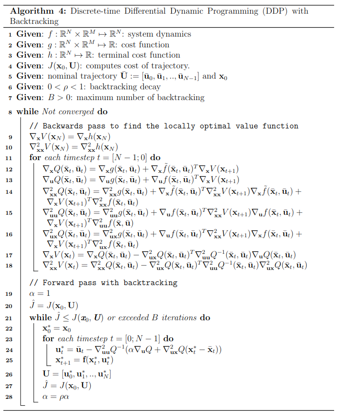
Since DDP is a second-order method, it makes large steps towards the solution and because we are approximating the underlying functions, it is often the case that we overshoot the minima when optimising non-convex functions. This leads to inefficient optimisation and sometimes completely unstable solutions. The figure below visualises how taking too large steps can make us completely overshoot the local minima (due to the approximative nature of Taylor series expansion).
![]()
To combat this, we can do some sort of line search to ensure that we are always making steps towards the minima. A popular and efficient method is backtracking where we scale back the solution if it results in a worse solution. For a simple 1D problem where we are trying to find the solution to a function $f$ with standard gradient descent, this looks like
Convergence criteria
We have a good idea of how to make an algorithm, but when do we stop optimising? In other words, what is our convergence criteria? There are multiple options for this, which are entirely empirically driven:
-
Cost reduction - if we label the cost of optimisation iteration $k$ as $J_k$ in the DDP algorithm, then we can create a convergence criteria based on $(J_k - J_{k+1})^2 < \epsilon$ where $\epsilon$ is a parameter we define. This method is straightforward and provides an overall good signal when further optimisation gives us diminishing returns.
-
Value gradient norm - another good way to estimate when we are very close to the optimal trajectory is by simply checking the gradients of our value function $\sum_{t=0}^{N} || \nabla_\textbf{x}V(\textbf{x}_t)||_2 < \epsilon$ where $\epsilon$ is again a parameter of our choice. This again is easy to compute and in theory gives us a more precise estimate if we are close to the local optima.
-
Time budget - not explicitly a convergence criteria but in practice when deploying DDP on robotics systems, we can’t afford to spend seconds to optimise a trajectory. Instead, we allocate a time budget per optimisation cycle. For example if we are running DDP in a receding horizon fashion at 10 Hz, then we have 0.1s to optimize between timesteps. After the 0.1s are out it doesn’t matter how optimal the trajectory is, we just need to execute it otherwise our robot might fall or drive off a cliff. Thus, in practice all of the convergence criteria above doesn’t make it into code, instead we try to optimise as much as we can within our allocated time budget.
Derivatives
Alright, you gave me this cool algorithm that can optimise trajectories with the power of linear algebra but there are so many derivatives everywhere, don’t tell me I have to compute them by hand?!? That is a nice exercise, but as with everything in modern times, we can just let computers figure it out. There are many ways that computers can compute derivatives:
-
Numerical differentiation - relies on the definition of derivative $f’(x) = \lim_{h \mapsto 0 } \dfrac{f(x+h) - f(x)}{h}$. If we take $h$ to be sufficiently small, then we can evaluate the function at two different points which gives us an estimate of the gradient. For this, we don’t even need to know the function $f$ but this is often inefficient (especially at higher dimensions).
-
Symbolic differentiation - manipulates a mathematical expression directly to obtain its exact derivatives. This is what you see Matlab or Wolfram Alpha do when you ask them to differentiate something. They compile the whole function as one big expression and compute it’s derivative following the same rules that we humans do - the product and chain rules.
-
Automatic differentiation - this is what powers modern deep learning libraries like Tensorflow and PyTorch. Imagine a big neural network that contains millions of math operations, compiling all of those into a single equation would be difficult (and possibly wouldn’t even fit in memory). Instead, automatic differentiation defines operations as nodes in a computational graph which we can traverse backwards to compute the gradients (backprop!).
What can we use for DDP? In principle, we can use all 3! In practice, it makes sense to use symbolic differentiation for simple low-dimensional functions eg. controlling a robot arm but if we are doing something more large scale, say optimizing a neural network with DDP (yes, you can do that) then it is more computationally efficient to use automatic differentiation.
In my implementation, I dealt with small robotic systems so I chose to use the marvellous sympy to get symbolic derivatives.
Experimental result
Inverted pendulum
I first apply DDP to the inverted pendulum problem from the deep mind control suite but with a modified state representation to deal with the angle wrap around issue. Namely, we use

State: $\textbf{x} = \begin{bmatrix} \sin(\theta) \ \cos(\theta) \ \dot{\theta} \end{bmatrix}$; Controls $\textbf{u} = \begin{bmatrix} \tau \end{bmatrix}$
Dynamics:
\[\dot{\textbf{x}} = \begin{bmatrix} \sin(\dot{\theta}) \\ \cos(\dot{\theta}) \\ \dfrac{-3g}{2L} \sin(\theta + \pi) + \dfrac{3}{mL^2} \tanh(u) \\ \end{bmatrix}\]Cost functions:
\[g(\textbf{x}, \textbf{u}) = (\textbf{x} - \textbf{x}_g)^T C (\textbf{x} - \textbf{x}_g) + \textbf{u}^T R \textbf{u}\] \[h(\textbf{x}_f) = (\textbf{x}_f - \textbf{x}_g)^T C_f (\textbf{x}_f - \textbf{x}_g)\]$\theta$ and $\dot{\theta}$ are the angle and angular velocity of the pendulum. We control it via torque $\tau \in [0; 1]$ which spins it in either direction. The control constraint is applied to the problem via the $tanh$ within the dynamics. Note that this is taken into account in the derivatives of the dynamics. $g, m, L$ are the gravity, mass and length parameters of the problem. $C$ and $R$ are the state and control cost matrices respectively. Note that they make the cost quadratic. I use a different matrix to weight the final state cost $C_f$. Applying DDP to this problem with trajectory length $N=100$ and timestep $\Delta t = 0.05s$, yields the results below. Code

Cartpole
Now we apply I to the slightly more complicated cartpole problem where we have a cart with a pole attached to it and the goal is to balance to pole upwards by only controlling the lateral force of the cart. We follow the problem definition and dynamics of defined by Ravzan Florian which is also used in the Deepmind control suite.
State: $\textbf{x} = \begin{bmatrix} x \ \dot{x} \ \sin(\theta) \ \cos(\theta) \ \dot{\theta} \end{bmatrix}$; Controls $\textbf{u} = \begin{bmatrix} \tau \end{bmatrix}$
The cost functions are quadratic as in the inverted pendulum problem. Similarly to before, using $N=100$ and $\Delta t = 0.05s$ we obtain the results shown below where we can see convergence to the locally optimal trajectory. Code

Acknowledgements
A kind thank you to Prof Evangelos Theodorou for giving me and supporting me with the exercise.