For decades, humans have been fascinated with controlling complex robots to do human-like dexterous skills. Building upon decades of control theory research, Boston Dynamics can make Atlas do some pretty cool things that only very few humans can do!
but why can’t Atlas do dishes, pick up drinking glasses, or sort groceries? Things that all humans do on a daily basis? I argue that classical control methods (such as MPC) don’t do well on contact-rich tasks. This is a major road-block to achieving human-level dexterous manipulation.
Possibly one of the (still) most impressive demos of dexterous robots is OpenAI’s robot hand solving Rubik’s Cube
How did a group of computer scientists do what roboticists couldn’t do for decades? They didn’t do it with classical control but with Reinforcement Learning (RL)! It turns out that RL is pretty good at learning through contact. It’s one of its more under-appreciated aspects that I want to dive into today.
Table of contents
- Why is contact hard?
- Gradient Types in Reinforcement Learning
- Optimizing through contact
- Conclusion
- References
Why is contact hard?
I can write hand-wavy paragraphs, trying to write down my thoughts, but that probably isn’t a good use of your time. Instead, let’s just look at a toy example!
Say we’re trying to throw a ball forward in free space for $t=2s$ and we want to maximize its forward distance travelled. I’ll label this optimization objective $J(\theta)$ where $\theta$ is the initial angle with respect to which we want to optimize our problem. From basic Newton physics, we can derive the objective and plot the resulting optimization landscape:
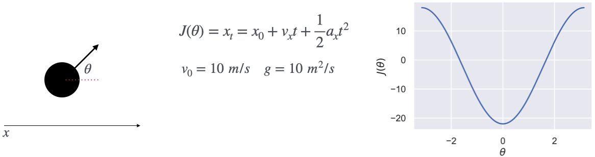
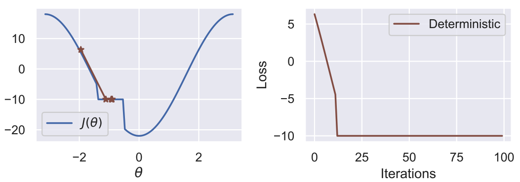
It looks pretty nice! We can just throw our favourite Gradient Descent (GD) optimizer at it. It’s going to do a pretty good job since the problem is smooth and mostly convex. However, what will happen if we erect a wall in front of the ball and assume that the ball just sticks to it when it hits it (i.e., no contact model)?
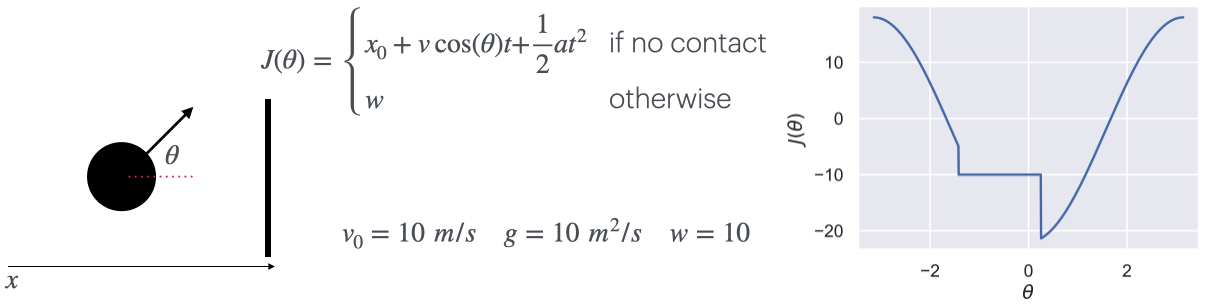
Hmm… gradient descent doesn’t look as good now. If we try optimizing this, we quickly run into a local minima:
Not great; how can we deal with this? A simple way is to make the problem stochastic by sampling our $\hat{\theta}$ from a Gaussian $\mathcal{N}(\theta, \sigma^2)$:
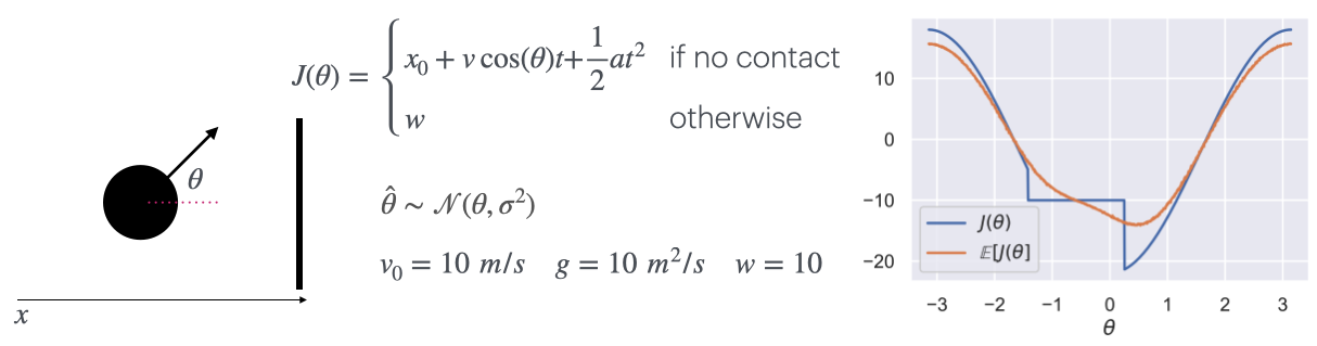
We call $\mathbb{E}[J(\theta)]$ the smooth surrogate of the real objective, and due to the added noise, it is smooth and much better behaved than the true objective! As a matter of fact, we can throw GD at it now!
Takeaway: Stochastic optimization helps us solve non-smooth tasks such as contact.
OK, how does this relate to the robot hand solving Rubik’s Cube? Let’s formalzie RL!
Gradient Types in Reinforcement Learning
Given a finite-horizon problem with state space $s_t \in \mathcal{S}$, actions $a_t \in \mathcal{A}$, rewards $r_t \in \mathbb{R}$ given by the reward function $r: \mathcal{S} \times \mathcal{A} \rightarrow \mathbb{R}$ and some dynamics function $f : \mathcal{S} \times \mathcal{A} \rightarrow \mathcal{S}$, we are interested in maximizing the cumulative reward:
\[\begin{equation} J(\theta) = \mathbb{E}_{\substack{ a_t \sim \pi_\theta(\cdot | s_t)}} \big[ \sum_{t=0}^T r(s_t, a_t) \big] \end{equation}\]where $\pi_\theta (\cdot | s_t)$ is our stochastic action policy, which we use to introduce noise into our problem.
Notes on formulation
Although it is atypical to deal with finite-horizon problems without considering starting state $s_0$, we make these simplifications to ease reading and derivation. It is easy to extend all results in this post to the infinite horizon case with some initial state distribution $\rho(s_0)$How can we solve this? i.e. $\max_\theta J(\theta)$. The most common way to do this in RL is via Policy Gradients (PG)!
Theorem 1: The gradient of Eq.1 can be estimated via Policy Gradients (PG) aka. score function, likelihood ratio, and zeroth-order gradients [1]:
\[\begin{equation} \nabla_\theta^{[0]} J(\theta) = \mathbb{E}_{ a_t \sim \pi_\theta(\cdot | s_t)} \bigg[ \bigg(\sum_{t=0}^H r(s_t, a_t) \bigg) \bigg(\sum_{t=0}^H \nabla_\theta \log \pi_\theta (a_t | s_t) \bigg) \bigg] \end{equation}\]- Doesn’t require us to know the $f(s,a)$, nor $r(s,a)$. We just need to be able to sample from them!
- Only need to know $\pi_\theta(a_t | s_t)$ and for it to bo continuously differentiable.
- Sample inefficient and has high variance.
- Only holds with expectation.
PGs are pretty cool! They allow us to solve things that we don’t know how to model! However, I want to focus on the final point - they only hold with expectation! In other words, PG can only be applied to stochastic problems, and stochastic problems smooth out discontinuities.
Great, but how do we actually compute Eq. 2? Expectations are nasty:
\[\nabla_\theta^{[0]} J(\theta) = \nabla_\theta \mathbb{E}_{\substack{ a_h \sim \pi(\cdot | s_h)}}{\sum_{h=1}^H r(s_h, a_h)} = \nabla_\theta \int \rho(s_1) \int \pi_\theta(a_h| s_h) r(s_h, a_h) \int (...) da_h ds_1\]That quickly becomes intractable for any reasonable problem. Can we make do with an estimate of the gradient?
Definition 1: Stochastic gradients can be estimated via Monte Carlo sampling, which we refer to as Monte Carlo Gradient Estimation [2]:
\[\begin{equation} \bar{\nabla}_\theta^{[\cdot]} J(\theta) = \dfrac{1}{N} \sum_{n=1}^N \hat{\nabla}_\theta^{[\cdot]} J(\theta)^{(n)} \end{equation}\]Note how I didn’t use the $[0]$ to indicate PGs. That is because I want to introduce another gradient type:
Definition 2: The gradient of objective Eq. 1 can be estimated with First-order Gradients (FOG) aka. pathwise gradients or the reparameterization trick:
\[\begin{equation} \nabla_{\theta}^{[1]} J(\theta) := \mathbb{E}_{a_h \sim \pi_\theta(\cdot | s_h)} \Big[ \nabla_\theta \sum_{h=1}^H r(s_h, a_h) \Big] \end{equation}\]These types of gradients:
- Assume known and differentiable $f(s,a), r(s,a), \pi(\cdot | s)$
- Are known to have less variance, thus being more sample efficient [1]
We now have 2 different types of gradients. How do we choose which one to use? There are a couple key properties we look for [1]:
- Consistency. As we increase the number of samples $N$ in Eq. 3, the gradient estimate should converge to the true gradient \(\bar{\nabla}_\theta J(\theta) \rightarrow \nabla_\theta J(\theta)\) as \(N \rightarrow \infty\). Both PG and FOG are consistent gradient estimators, as proven by the Law of Large Numbers [2].
- Computational efficiency. Ultimately, we are interested in obtaining the best gradient estimates in a unit of wall-clock time. This can materialize as using fewer MC samples, scalability to parameter dimensionality $d$, the unit cost of computing gradients, or computations that can be easily parallelized. This topic is ultimately empirical and out the scope of this blog.
- Bias. If we repeat the estimation process many times, will our estimates be centred on the true value of the gradient? In other words, what is the accuracy of the gradient estimates for varying N?
- Variance. Any estimator using Eq. 3 is a random variable. All other things being equal, we always prefer an estimator with a lower variance as it enables more efficient learning.
Let’s first handle the topic of bias, about which we can say a lot of things theoretically!
Assumption 1: To ensure $\nabla J(\theta)$ is well defined, we assume that the policy $\pi_\theta ( \cdot | s)$ is continuously differentiable $\forall s \in \mathbb{R}^n, \forall \theta \in \mathbb{R}^d$. Furthermore, the system dynamics $f$ and reward $r$ have polynomial growth.
Lemma 1: Under Assumption 1, PG is an unbiased gradient estimator of the stochastic objective [3]:
\[\begin{equation} \mathbb{E} \big[ \bar{\nabla}^{[0]} J(\theta) \big] = \nabla J(\theta) \end{equation}\]Assumption 2: The system dynamics $f(s, a)$ and the reward $r(s, a)$ are continuously differentiable $\forall s \in \mathbb{R}^n, \forall a \in \mathbb{R}^m$.
Lemma 2: Under Assumptions 1 and 2 and if $f(s, a)$ and $r(s, a)$ are Lipschitz smooth, then FOG are almost surely defined and unbiased [3]:
\[\begin{equation} \mathbb{E} \big[ \bar{\nabla}^{[1]} J(\theta) \big] = \nabla J(\theta) \end{equation}\]Takeaway: Both PGs and FOGs can be unbiased gradient estimators but FOGs require more assumptions.
Optimizing through contact
Saying things about variance is a bit more tricky, so we will explore it empirically by comparing the gradient types in our toy examples.
First, let’s look at the example of the ball being thrown in free space (i.e., no wall). We can actually quite easily compute the true analytical gradient:
\[J(\theta) = \mathbb{E}_{\substack{ a_h \sim \pi(\cdot | s_h)}}{\big[ x_0 + v \cos(\theta) t + \dfrac{1}{2}a t^2} \big] \quad \quad \quad \hat{\theta} \sim \pi_\theta(\cdot) = \mathcal{N}(\theta, \sigma^2)\] \[\nabla_\theta \mathbb{E}_{w \sim \mathcal{N}(0, \sigma^2)} \big[ {-x_0 - v cos(\theta + w) t + \dfrac{1}{2} t^2} \big] = \dfrac{vt}{\sqrt{2}} \exp(\dfrac{-\sigma^2}{4}) \sin(\theta)\]Where we exploit the fact that $\hat{\theta} = \theta + w$ where $w \sim \mathcal{N}(0, \sigma^2)$
Computing gradients with a low $N=50$ (realistic value) while varying noise $\sigma$ reveals hopefully an obvious result:
- Under small (/useful) $\sigma$, FOG have lower variance and bias
- FOG variance scales linearly with $\sigma$
- PG variance remains fairly consistent with $\sigma$
Takeaway: If everything is smooth, FOGs are almost always better
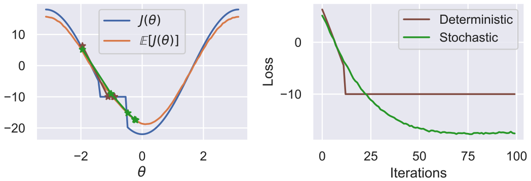
Let’s now make things a bit more interesting by erecting a wall again! This transforms our problem into:
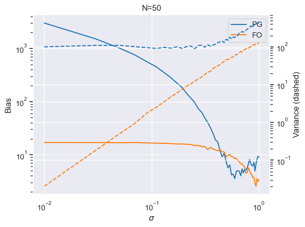
\[J(\theta) = \mathbb{E}_{\substack{a_h \sim \pi(\cdot | s_h)}} \begin{cases} x_0 + v \cos(\theta) t + \dfrac{1}{2} a t^2 & \text{if no contact} \\ w & \text{otherwise} \end{cases} \quad \quad \quad \hat{\theta} \sim \pi_\theta(\cdot) = \mathcal{N}(\theta, \sigma^2)\]Our problem now becomes discontinuous and is heavily affected by the level of smoothing $\sigma$ and the number of samples $N$:
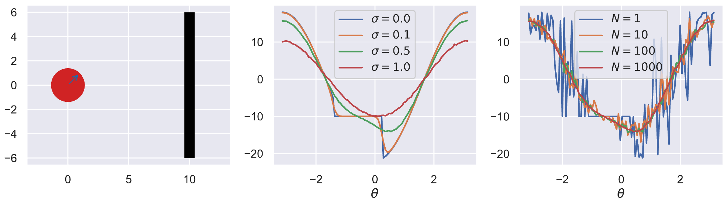
Where in the middle plot we see the true objective $J(\theta)$. Investigating the bias-variance trade-off in the same fashion as before reveals more interesting results:
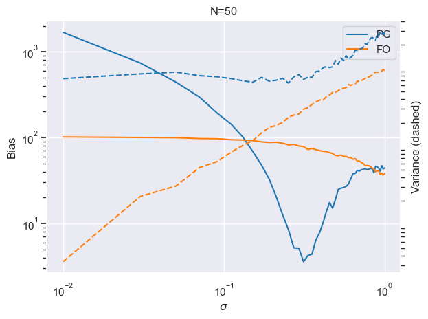
Things are less clear-cut now:
- FOG bias has increased by an order of magnitude, while PG bias has reduced! We actually have a word for this type of FOG bias - empirical bias. [3]
- For the spectrum of useful $\sigma$, PGs have a lower bias.
- FOG variance has increased by an order of magnitude, while PG has remained similar.
However, that is not all, PGs have one more trick up their sleeve! A variance reduction technique called baseline subtraction:
\[\nabla_\theta^{[0]} J(\theta) := \mathbb{E}_{a_h \sim \pi_\theta(\cdot | s_h)} \Bigg[ {\big( \sum_{h=1}^H r(s_h, a_h) - \color{red} \sum_{h=1}^H r(s_h, \mathbb{E} [a_h]) \color{black} \big) \big( \sum_{h=1}^H \nabla_\theta \log \pi_\theta(a_h | s_h)} \big) \Bigg]\]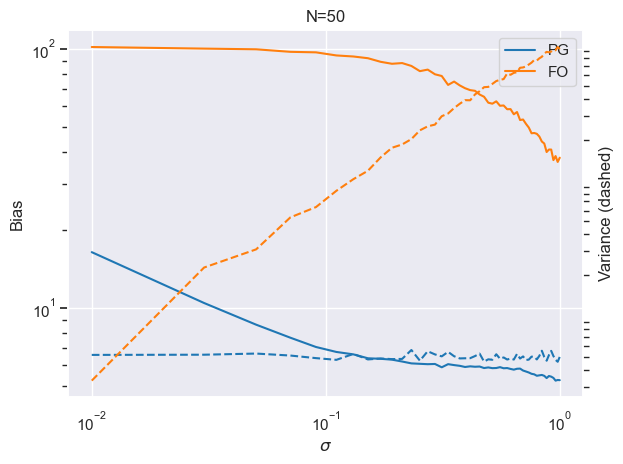
Takeaway: For heavily discontinuous problems, PGs are almost always better
We can also do some theoretical analysis on these results:
Lemma 3: If the policy $\pi$ is $B_\pi$-Lipshitz, then PG variance can be bounded by:
\[\begin{align} \mathbb{V} \big[ {\bar{\nabla}^{[0]} J(\theta)} \big] = \dfrac{1}{N} \mathbb{V} \big[ {\hat{\nabla}^{[0]}J_i(\theta)} \big] \leq \dfrac{1}{N \sigma^2} B^2_\pi n \end{align}\]Most importantly, the variance of PG estimates is not bound by the objective function. PG exhibit the same variance when applied to either smooth or non-smooth objective functions. Proof can be found in [3].
Lemma 4: If the policy $\pi$ is $B_\pi$-Lipshitz, the reward $r(\cdot, \cdot)$ is $B_r$-Lipshitz and the dynamics $f(\cdot, \cdot)$ are $B_f$-Lipshitz, then the variance of FOG can be bounded by:
\[\mathbb{V} \big[ {\bar{\nabla}^{[1]} J(\theta)} \big] = \dfrac{1}{N} \mathbb{V} \big[ {\hat{\nabla}^{[1]}J_i(\theta)} \big] \leq \dfrac{1}{N\sigma^2} B_r^2 B_\pi^2 B_f^2 m\]Unlike PG, these types of gradients are bound by the smoothness of the objective function expressed via $B_\pi$ and $B_f$. Crucially, the less smooth our objective is, the higher the variance. Proof can be found in [4].
Lemma 5: For a stochastic optimization problem under Assumption 1, which also has $B_\pi$-Lipshitz smooth policy $\pi$ and Lipshitz-smooth and bounded rewards $r(s, a) \leq ||\nabla r(s, a)|| \leq B_r$ $\forall s \in \mathbb{R}^n; a \in \mathbb{R}^m; theta \in \mathbb{R}^d$, then PGs remain consistently unbiased. However, FOGs exhibit bias bounded by:
\[\| \mathbb{E} \big[ {\nabla_\theta^{[1]} J(\theta)} \big] - \mathbb{E} \big[ {\nabla_\theta^{[0]} J(\theta)} \big] \| \leq B_r^2 B_\pi^2 \mathbb{E} \big[ \| \nabla f(s, a) \|^2 \big]\]$B_r$ can be bounded via reward engineering. $B_\pi$ can be bounded by engineering a nice policy. However, the dynamics are more difficult to bound as they are naturally discontinuous. Not great for FOGs. We call this the empirical bias of FOGs! Proof can be found in [4].
Conclusion
Let’s circle back. What makes RL tick? Why has it been able to do what classical optimal control hasn’t been able to, especially relating to contact-rich robot tasks?
The main reason is the Policy Gradients Theorem, which is surprisingly robust to discontinuities, but the more subtle and less appreciated reason is the fact that the theorem requires stochastic optimization which in turn smooths out the underlying optimization landscapes.
The key takeaways I want you to get from this blog post are:
- Stochastic optimization helps us solve non-smooth tasks.
- If everything is smooth, FOGs are almost always better.
- If dynamics aren’t smooth and we need objective smoothing, PGs are better.
For more practical robotics applications, we want to use PGs when in contact and FOGs when not in contact. For contact-rich tasks such as the OpenAI Rubik’s Cube task, we might as well just use PGs altogether.
Thank you for making it this far. I hope that you learned something!
If you have any comments or suggestions, shoot me an email!
References
- [1] Mnih et al., Monte Carlo Gradient Estimation in Machine Learning
- [2] Robert et al., Monte Carlo statistical methods
- [3] Suh et al., Do Differentiable Simulators Give Better Policy Gradients?
- [4] Georgiev et al., Adaptive Horizon Actor-Critic for Policy Learning in Contact-Rich Differentiable Simulation